


Support vector machines (SVMs) are a great machine learning tool for predictive modeling. In this post, I illustrate how to use them. For most problems SVMs are a black box: you select your outcome variable and predictors, and let the algorithm work its magic. The key thing that you need to be careful about is overfitting, so this is my focus.
Overfitting is one of the greatest challenges faced when training a model to predict outcomes. In this blog post I show how to split data into a training and testing set, then how to fit support vector machines to the training set and assess their performance with the testing set. I use data about that delicious (for some), marine mollusc with brightly colored inner shells, the abalone. Our aim is to predict their gender from other physical characteristics. One peculiar feature of abalone that concerns us here is that infants have undetermined gender, hence the outcome variable has 3 categories and not 2.
Splitting the data and training the model
First, we need to randomly split the data into a larger 70% training sample and a smaller 30% testing sample. In Displayr we do this with Insert > Utilities > Filtering > Filters for Train-Test Split. This creates 2 new variables which can be used as filters. We are going to use the training sample to try different values of the support vector machine cost parameter and then check our models with the test sample.
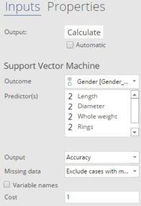
In Displayr we add a support vector machine via Insert > More > Machine Learning > Support Vector Machine. I’ve chosen Length, Diameter, Whole weight and Rings as the Predictor variables, and Gender as the Outcome. The other settings are left to their defaults as shown on the right. Finally to restrict the model to the training set, I change the filter (Home > Filter (Data Selection)) to Training sample. The result gives an overall accuracy of 56.77%, with a better performance for males and infants than females (as indicated by the bars).
Predicting with the test data
Although we now know the accuracy for predicting the genders in the training data, of more relevance is the accuracy on the 30% of the data that the support vector machine has not seen – the testing sample. To calculate this:
- Select the output from the support vector machine.
- Select Insert > More > Machine Learning > Diagnostic > Prediction-Accuracy Table.
- With the prediction accuracy table selected, choose the Testing sample filter in Home > Filter (Data Selection).
The prediction-accuracy table illustrates the overlap between the categories which are predicted by the model and the original category of each case within the testing sample. The accuracy drops to 52.51%, as shown beneath the chart. The reduction is no surprise since the model has not seen this data before. Can we improve the performance of a support vector machine on unseen data?
Optimizing the cost
The cost parameter of a support vector machine determines how strictly it fits the training data. A high cost means the model attempts to make correct predictions on the training data even if that implies a complex relationship between the predictor and target variables. By contrast a low cost produces a simple model that is more prone to making mistakes on the training data. Higher cost leads to better accuracy on the training data, as shown in the table below. However this is not what we should be optimizing, rather we should aim to improve the accuracy on unseen data. Note that is it usual to explore a wide range of costs in a multiplicative manner, for example by increasing/decreasing in powers of 10. In Displayr, the cost parameter can be modified in the options for the support vector machine output (as shown in the screenshot above).
By increasing the cost we discover that test accuracy peaks at close to 55% with a cost of 1,000, then drops for higher values. This is overfitting in action. Predictions on the testing set are deteriorating at such high costs because the model is paying too much attention to aspects of the training data that are in fact random and do not help generalize to unseen examples. Looking at the test accuracy allows us to identify the point where the model has learned the essence of the relationship between the predictor and outcome variables but is not so focused that it is simply memorizing the training data. Another side-effect of high costs is that the model takes longer to run due to its complexity.
At the other end of the scale a cost of 0.001 leads to 37% testing accuracy and the Prediction-Accuracy Table shows that the model is so simple it predicts everything to be male, the most frequent category. This is underfitting – the patterns of the data have not been learned well enough to make good predictions.
For the best performance we avoid both overfitting and underfitting, in this case with a cost of 1000.
TRY IT OUT
You can explore this data set for yourself in Displayr.
Photo credit: schoeband via VisualHunt.com / CC BY-NC-ND