
In decision trees, the best split at each node is determined by evaluating how well each potential division separates the data, using criteria like Gini impurity, entropy, or sum of squared errors. This post will explain how these splits are chosen.
If you want to create your own decision tree, you can do so using this decision tree template.

What Is a Decision Tree and How Does It Work?
This post builds on the fundamental concepts of decision trees, which are introduced in this post.
Decision trees are trained by passing data down from a root node to leaves. The data is repeatedly split according to predictor variables so that child nodes are more “pure” (i.e., homogeneous) in terms of the outcome variable. This process is illustrated below:
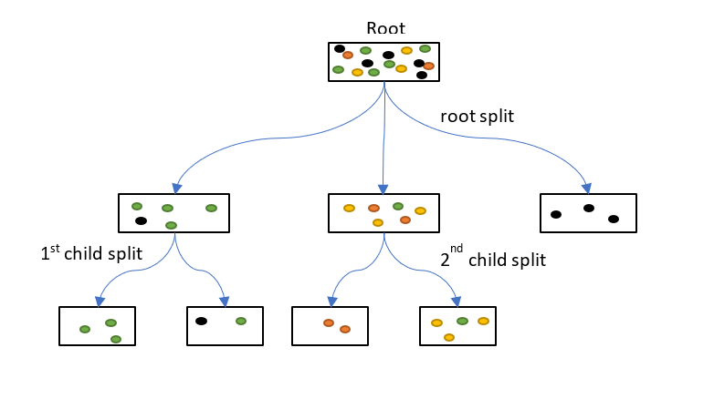
The root node begins with all the training data. The colored dots indicate classes which will eventually be separated by the decision tree. One of the predictor variables is chosen to make the root split. This creates three child nodes, one of which contains only black cases and is a leaf node. The other two child nodes are then split again to create four more leaves. All the leaves either contain only one class of outcome, or are too small to be split further.
At every node, a set of possible split points is identified for every predictor variable. The algorithm calculates the improvement in purity of the data that would be created by each split point of each variable. The split with the greatest improvement is chosen to partition the data and create child nodes.
How Are Split Points Chosen in a Decision Tree?
The set of split points considered for any variable depends on whether the variable is numeric or categorical. The values of the variable taken by the cases at that node also play a role.
When a predictor is numeric, if all values are unique, there are n – 1 split points for n data points. Because this may be a large number, it is common to consider only split points at certain percentiles of the distribution of values. For example, we may consider every tenth percentile (that is, 10%, 20%, 30%, etc).
When a predictor is categorical we can decide to split it to create either one child node per class (multiway splits) or only two child nodes (binary split). In the diagram above the Root split is multiway. It is usual to make only binary splits because multiway splits break the data into small subsets too quickly. This causes a bias towards splitting predictors with many classes since they are more likely to produce relatively pure child nodes, which results in overfitting.
If a categorical predictor has only two classes, there is only one possible split. However, if a categorical predictor has more than two classes, various conditions can apply.
If there is a small number of classes, all possible splits into two child nodes can be considered. For example, for classes apple, banana and orange the three splits are:
| Child 1 | Child 2 | |
|---|---|---|
| Split 1 | apple | banana, orange |
| Split 2 | banana | apple, orange |
| Split 3 | orange | apple, banana |
For k classes there are 2k – 1 – 1 splits, which is computationally prohibitive if k is a large number.
If there are many classes, they may be ordered according to their average output value. We can the make a binary split into two groups of the ordered classes. This means there are k – 1 possible splits for k classes.
If k is large, there are more splits to consider. As a result, there is a greater chance that a certain split will create a significant improvement, and is therefore best. This causes trees to be biased towards splitting variables with many classes over those with fewer classes.
Types of Decision Tree Split Criteria (Gini, Entropy, SSE)
At the core of every decision tree split is a mathematical criterion used to evaluate how “pure” the resulting child nodes are. The most common split criteria depend on whether the outcome variable is categorical or numeric:
- Gini Impurity: Measures how often a randomly chosen element from the set would be incorrectly labeled if randomly assigned a label according to the distribution of labels in the node. It’s fast to compute and widely used in classification tasks.
- Cross-Entropy (a.k.a. Information Gain): Another popular criterion for classification. It measures the uncertainty in the dataset and how much that uncertainty is reduced after the split.
- Sum of Squared Errors (SSE): Used when the outcome is numeric. It calculates the difference between the actual and predicted values and favors splits that reduce this difference.
Each of these metrics helps the tree decide which variable and which value (or grouping) offers the most meaningful separation at that point in the tree.
How Is the Best Split Determined at Each Node?
When the outcome is numeric, the relevant improvement is the difference in the sum of squared errors between the node and its child nodes after the split. For any node, the squared error is:
\[
\sum_{i=1}^{n}{(y_i-c)}^2
\]
where n is the number of cases at that node, c is the average outcome of all cases at that node, and yi is the outcome value of the ith case. If all the yi are close to c, then the error is low. A good clean split will create two nodes which both have all case outcomes close to the average outcome of all cases at that node.
When the outcome is categorical, the split may be based on either the improvement of Gini impurity or cross-entropy:
\[
Gini\ impurity=\sum_{i=1}^{k}{p_i(1-p_i)}
cross-entropy=-\sum_{i=1}^{k}{p_ilog(p_i)}
\]
where k is the number of classes and pi is the proportion of cases belonging to class i. These two measures give similar results and are minimal when the probability of class membership is close to zero or one.
Example: How a Decision Tree Calculates the Best Split
For all the above measures, the sum of the measures for the child nodes is weighted according to the number of cases. An example calculation of Gini impurity is shown below:
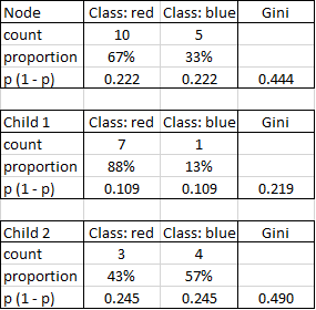
The initial node contains 10 red and 5 blue cases and has a Gini impurity of 0.444. The child nodes have Gini impurities of 0.219 and 0.490. Their weighted sum is (0.219 * 8 + 0.490 * 7) / 15 = 0.345. Because this is lower than 0.444, the split is an improvement.
One challenge for this type of splitting is known as the XOR problem. When no single split increases the purity, then early stopping may halt the tree prematurely. This is the situation for the following data set:
Why Decision Trees Prefer Variables with More Categories
One lesser-known challenge in decision tree construction is split bias. This is the tendency for trees to favor variables with more unique values or categories.
When a variable has many possible classes (e.g., a “Product” field with 20 different items), there are simply more ways to divide the data. This increases the likelihood of finding a split that appears statistically “good,” even if the variable isn’t truly predictive.
This is especially problematic with categorical predictors, where the number of possible binary splits grows rapidly with each additional class. For example, a variable with 10 categories has 511 possible binary splits.
As a result, decision trees may overfit by repeatedly selecting high-cardinality variables, leading to less generalizable models. To mitigate this, some algorithms adjust for variable cardinality or use pruning techniques to avoid overfitting.
You can make your own decision trees in Displayr by using the template below.