


What is an alternative-specific design?
The most common example of an alternative-specific design is a transport choice experiment. In each question, respondents choose between alternative methods of travel to work, such as Walk, Drive and Bus. A typical question would be to choose between three alternatives, such as those shown below.
Note that the attributes are different for each alternative. Drive has a Parking attribute that is not shown for Walk and Bus. Alternative-specific design are used in such situations where the attributes that describe some alternatives do not apply to other alternatives. Often this arises with labelled alternatives, i.e. where each attribute label is shown exactly once per question. This is in contrast to a standard choice experiment, for instance choosing between sports drinks where each drink has the same attributes of cost, color, sugar content and bottle size.
An example design
Before going any further, you might want to look at this Displayr document where you can follow my steps and try them for yourself. Continuing with the transport example, let’s consider an experiment with the following alternatives,
- Walk with one attribute:
- Travel time with three levels (30 mins, 40 mins, 50 mins)
- Drive with two attributes:
- Travel time with three levels (10 mins, 15 mins, 20 mins)
- Parking with four levels ($2, $5, $10, $20)
- Bus with three attributes:
- Travel time with three levels (20 mins, 25 mins, 30 mins)
- Wait time with four levels (0 mins, 5 mins, 10 mins, 15 mins)
- Crowding with three levels (Empty, Half full, No seats)
Not only are there attributes which are specific to certain alternatives, but the same attribute can have different levels per alternative. Hence Walk shows more appropriate longer travel times than Drive. Although they are labelled the same, each mode of transport has its own Travel time attribute.
Design algorithms
There are two approaches to making an alternative-specific design.
- Random – A simple and fast algorithm. As the name implies, for each question a random level is chosen for every attribute of every alternative.
- Federov – Named after its inventor, this procedure starts with a random design which is sequentially improved by trying different questions until no more improvement is found. Federov is slower than Random but produces a more balanced design where the number of appearances of each level is more consistent. Technically, the algorithm is optimizing the D-error of the design.
Creating the design in Displayr
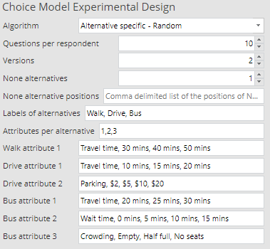
In Displayr, a choice model design is created by navigating to the Insert tab and clicking on More > Conjoint/Choice Modeling > Experimental Design. An example of the inputs is shown below. Besides the Algorithm as already described, the usual choice model inputs of Questions per respondent, Versions and None alternatives are specified.
The alternatives are defined by a comma-separated list of labels. In Attributes per alternative, another comma-separated list provides the number of attributes of each alternative (in the same order as the alternative labels).
Each of the following boxes contains a comma-separated list of the attribute label, followed by its levels. For example, the first such box, Walk attribute 1, shows that the label of this attribute is Travel time and its levels are 30 mins, 40 mins and 50 mins.
The table below shows an example of one question. Each row represents an alternative, where the 4th row is the None alternative and so is blank. Attributes that are not part of a certain alternative (e.g. Drive.Travel time in the first row) are also blank.
Maximum candidate questions
Earlier I mentioned that the Federov algorithm tries different questions in order to optimize the design. The number of possible questions of a design is the product of the numbers of alternatives there are for each level. For the design above this makes 3 * 3 * 4 * 3 * 4 * 3 = 1,296 potential different questions. Since there are two versions in the design, the number of questions that are examined is multiplied by a factor of 2, i.e., 2592, as the algorithm considers a separate set of candidate questions for each version.
Designs can easily be much larger, with many more alternatives, attributes, levels and versions. This means that the number of possible questions can run into the billions, which poses a computational problem. Examining such a large number of questions is infeasible in a realistic time frame.
This is where the Maximum candidate questions box is used. Setting Maximum candidate questions limits the number of questions that are examined during the optimization process. This is useful if the Federov algorithm is taking too long. Naturally this means that the design might not be as optimal as when all questions are considered, but it will certainly be necessary for very large designs unless you are prepared for a very long wait. I suggest starting with 100,000 candidates (which are chosen randomly from all possible questions) and iterating from there depending on how much time you can spend.
Comparison of designs
To the diagnostics for the design are conveniently included at the top of the output, which is shown for the Random example design below.
The first value shown is D-error. D-error is a measure that shows how good or bad a design is at extracting information from respondents. A lower D-error indicates a better design. Usually, D-errors are used to compare the quality of designs created by different algorithms. The corresponding value for the Federov algorithm is 5.61.
The following rows, singles, show tables of the frequency of occurrence of each level. Since this is a random design there are significant fluctuations. For example, in the Crowding attribute of the Bus alternative Half full is shown 11 times but Empty is shown only twice.
Finally, pairs show tables of the co-occurrence of the levels for each pair attributes of an alternative. These numbers also show a large amount of variation. The same tables for the Federov algorithm are much more balanced.
Read more about market research, or try this analysis yourself!