

Residuals in a statistical or machine learning model are the differences between observed and predicted values of data. They are a diagnostic measure used when assessing the quality of a model. They are also known as errors.
What Are Residuals in Statistics?
Put simply, residuals are the differences between the observed values in your dataset and the values predicted by a statistical or machine learning model. Here’s the formula (if you really want to simplify it):
Residual = Observed – Predicted.
So why do we use residuals in statistics? Well, they tell us how far off the model’s prediction is from reality, and are essential for diagnosing the accuracy and reliability of your model. If all residuals are close to zero, your model is likely performing well. Larger or patterned residuals may point to deeper problems.
Example of Residuals in a Real Model
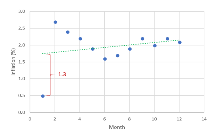
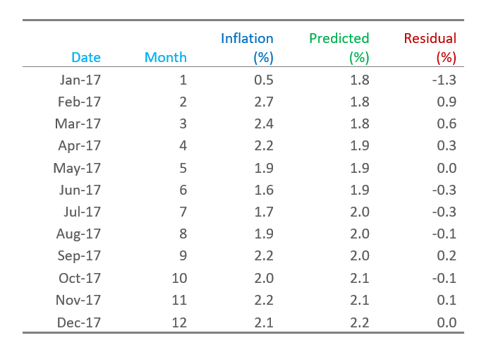
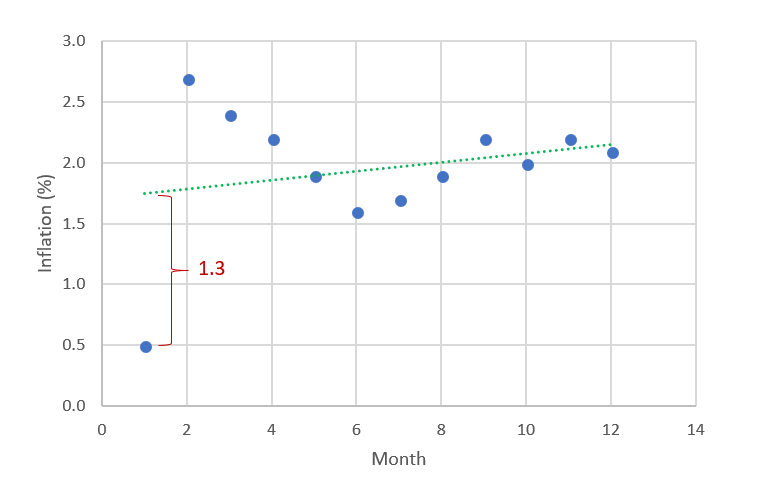
The middle column of the table below, Inflation, shows US inflation data for each month in 2017. The Predicted column shows predictions from a model attempting to predict the inflation rate. The residuals are shown in the Residual column and are computed as Residual = Inflation – Predicted. In the case of the data for January 2017, the observed inflation was 0.5%, the model has predicted 1.8%, so the residual is –1.3%.
The chart below shows the data in the table. You can read the residuals as being the difference between the observed values of inflation (the dots) and the predicted values (the dotted line).
Residuals Meaning and Interpretation
Residuals are important when determining the quality of a model. You can examine residuals in terms of their magnitude and/or whether they form a pattern.
Where the residuals are all 0, the model predicts perfectly. The further residuals are from 0, the less accurate the model. In the case of linear regression, the greater the sum of squared residuals, the smaller the R-squared statistic, all else being equal.
Where the average residual is not 0, it implies that the model is systematically biased (i.e., consistently over- or under-predicting).
Where residuals contain patterns, it implies that the model is qualitatively wrong, as it is failing to explain some property of the data. The existence of patterns invalidates most statistical tests.
Residual Statistics: How They Work in Models
Residuals aren’t just raw errors – they’re a statistical tool used to evaluate the fit and assumptions of a model. Analysts examine the size, direction, and pattern of residuals to assess bias, variance, and structural flaws.
In linear regression, for example, the sum of squared residuals directly influences the R-squared value. Clean, pattern-free residuals indicate that the model is capturing the data well. Residual analysis is common in model selection, validation, and optimization workflows.
Common Residual Problems and How to Diagnose Them
If some of the residuals are relatively large compared to others, either the data or model may be flawed. The next step is to investigate and work out what has specifically led to the unusually large residual.
In the example above, the residuals for January and February are much further from 0 than the residuals for the other months. Thus, it may be worthwhile to investigate what was unusual about January. Unusually large residuals are called outliers or extreme values.
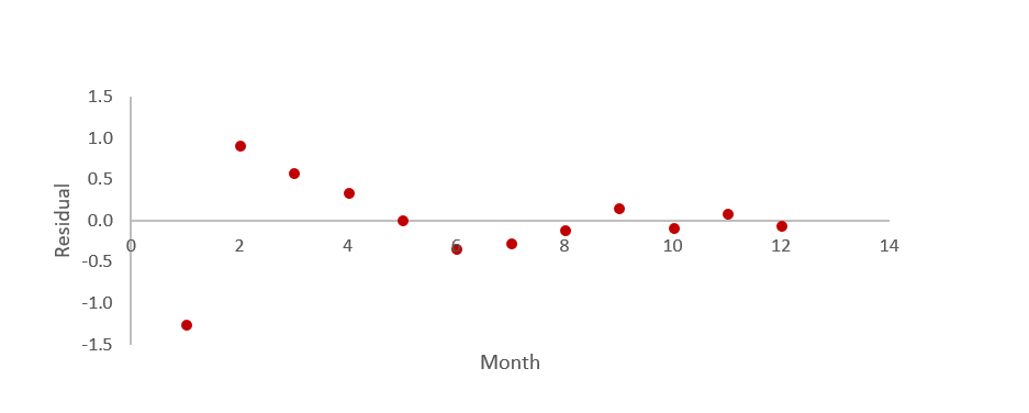
Another common type of pattern in residuals is when we can predict the value of residuals based on the preceding values of residuals. This phenomenon is known by various names, including autocorrelation, serial correlation, and serial dependence. The residuals in this case to seem to have a snake-like pattern – evidence of autocorrelation.
Another type of pattern occurs when the degree of variation in the residuals appears to change over time. This pattern is known as heteroscedasticity. In the plot above, we can see some evidence of heteroscedasticity, with residuals in months 1 through 4 being further from 0 than the residuals from months 5 through 12.
Another type of pattern relates to the distribution of the residuals. In some situations, it can be informative to see if the residuals are distributed in accordance with the normal distribution.
Different Types of Residuals Explained
Sometimes residuals are scaled (i.e., divided by a number) to make them easier to interpret. In particular, standardized and studentized residuals typically rescale the residuals so that values of more than 1.96 from 0 equate to a p-value of 0.05. Different software packages use terminology inconsistently. Additionally, most packages do not account for multiple comparison correction errors, so be cautious when interpreting documentation that uses scaled residuals.
FAQs About Residuals
What’s the difference between residuals and errors?
Residuals are the difference between observed and predicted values in your sample data. Errors refer to the difference between actual values and model predictions in the entire population, which we typically can’t observe directly.
Are residuals always normally distributed?
Not always. In many models, such as linear regression, residuals are assumed to be normally distributed; however, this assumption must be verified using visual tests, such as histograms or Q-Q plots.
How do I calculate residuals in Excel?
To calculate residuals in Excel, subtract the predicted values from the observed values using a simple formula: =Observed - Predicted. Do this for each row of your data.
Head on over to the Displayr blog to find out more about all things data science and machine learning.