Customization of Bubble Charts for Correspondence Analysis in Displayr

When you insert a bubble chart in Displayr (Insert > Visualization > Bubbleplot), you can customize some aspects of its appearance from the controls that appear in the object inspector on the right of the screen. More advanced customizations can be performed by instead inserting an R Output (Insert > R Output), and writing code. I illustrate this by explaining how I created the visualizations in my Using Bubble Charts to Show Significant Relationships and Residuals in Correspondence Analysis, shown below.
The visualization above is shown at the end of the post. It is created by a quite lengthy chunk of code. Fortunately, you do not need to understand all of it! In this post I walk through some of the key steps of customizing bubble charts by modifying this code.
Create your Bubble Plot
Hooking up the code (not as scary as it looks)
The code below creates a correspondence analysis, and then presents this using a bubble chart. To reproduce a similar visualization with your own data:
- Create a table in Displayr that contains the data you want to analyze. This is no different to when you would normally do correspondence analysis.
- Select the table and you can see the Name of the table in the Object Inspector > Properties > GENERAL. When I did this, the name of my table was table.Q9.
- Click on the page containing the table in the list of Pages (far-left of the screen), and select Home > Duplicate, which will create a new page that contains the same table again.
- Click on the table on the new page, and select Object Inspector > Inputs > STATISTICS > Statistics - Cells and choose z-Statistic. Repeat this process to de-select %.
- Click on the table and change the name of the table in Object Inspector > Properties > GENERAL > Name to table.zScores (or anything else you want).
- Insert > R Output and paste in the code below, modifying the first 12 lines as per your needs. In the first line you replace table.Q9 with the name of your table (see step 2). In the 3rd line you replace Egypt with the name of the row that contains the standardized residuals that you wish to use, filling in the other rows with the labels that you wish to have appear on the final visualization.
 x = table.Q9
z = table.zScores
row.to.use = "Egypt"
row.label = "Country"
column.label = "Concern"
title = "Traveler's concerns about different countries (bubbles relate to Egypt)"
legend.title = "Strength of relationship"
# Removing rows and columns to be ignored
remove = c("NET", "Total")
x = x[!rownames(x) %in% remove, !colnames(x) %in% remove]
z = z[row.to.use, !colnames(z) %in% remove]
colnames(x) = paste0(colnames(x), ": ", round(x[row.to.use,]), "%")
# Default circle size (this is relative to the z-scores)
z[abs(z) <= 1.96] <- 0 #This turns off the significance.
default.size = 0.1 # Minimum circle size
my.ca = ca::ca(x)
coords = flipDimensionReduction::CANormalization(my.ca, "Principal")
n.rows = nrow(coords$row.coordinates)
n.columns = nrow(coords$column.coordinates)
coords = rbind(coords$row.coordinates, coords$column.coordinates)
# Creating the 'group' variable
n = n.rows + n.columns
groups <- rep("No association", n.columns)

groups[z > 0] = paste0("Weakness of ", row.to.use)
groups[z < 0] = paste0("Strength of ", row.to.use)
groups <- c(rep(row.label, n.rows), groups)
# Setting bubble size
bubble.size <- c(rep(default.size, n.rows), abs(z))
# Labeling the dimensions
singular.values <- round(my.ca$sv^2, 6)
variance.explained <- paste(as.character(round(100 * prop.table(singular.values), 1)), "%", sep = "")[c(1, 2)]
column.labels <- paste("Dimension", c(1, 2), paste0("(", variance.explained, ")"))
bubble.size[bubble.size < default.size] <- default.size
rhtmlLabeledScatter::LabeledScatter(X = coords[, 1],
Y = coords[, 2],
Z = bubble.size,
label = rownames(coords),
label.alt = rownames(coords),
group = groups,
colors = c("Black", "Purple", "#FA614B", "#3E7DCC"),
fixed.aspect = TRUE,
title = title,
x.title = column.labels[1],
y.title = column.labels[2],
z.title = legend.title,
axis.font.size = 10,
labels.font.size = 14,
title.font.size = 20,
legend.font.size = 15,
y.title.font.size = 16,
x.title.font.size = 16)
Turning off the significance testing
The visualization below is the same as the one above, except that the significance testing has been turned off. This was achieved by:
- Commenting out line 14 (i.e., typing a # at the very beginning of the line, which prevents that line of code being run).
- Removing , "purple" from line 40 and swapping around the order of the two last colors ( "#3E7DCC", "#FA614B"). This is where you customize the colors. You can type in a color code, or a color name, such as "Red" or "Blue".
Only showing the positive residuals
The next plot shows only the positive residuals (i.e., the concerns about Egypt that have the strongest relationship). It was created by:
- Removing the three letters abs from line 28.
- Commenting out line 25.
- In line 40, replacing #3E7DCC with Purple.
Taking the data values off the chart
Lastly, to remove the percentages from the visualization, comment out line 12, which leaves us with the visualization below.
More advanced customizations
If you hover your mouse over the word LabeledScatter in Properties > R CODE (line 34), a tooltip shows all the definitions of the parameters in this function, which allow further customization to be performed.