A well-known problem with linear regression, binary logit, ordered logit, and other GLMs, is that a small number of rogue observations can cause the results to be misleading. For example, with data on income, where people are meant to write their income in dollars, maybe one person writes their income as 50, meaning $50,000, and a billionaire may also include their much larger income. In this post I describe how you can automatically check for, and correct for, such problems in data. Such rogue observations have various different names, such as outliers and influential observations.
How to detect rogue observations
There are two basic stages of detecting rogue observations. The first is to create and inspect summary plots and tables of your data prior to fitting a model. The second is to use automatic tests that check to see if there are any observations that, when deleted from the data used to fit the model, cause the conclusions drawn from the model to change.
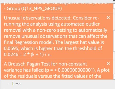
In Displayr and Q various standard techniques are used to see if there are any rogue observations. If detected, they appear as warnings, like the one shown below. If new to statistics, the warnings can be a bit scary at first. Sorry! But, do take the time to process them, once you get over the scariness, you will grow to appreciate that they are structured in a useful way.
The first thing to note is that one reason that they are scary is that they are written in very precise language. Rather than say “yo, look here, we’ve got some rogue observations”, they are using the correct statistical jargon, which in this case is that the rogue observations are influential observations. This is due to the fact it’s referring to the hat values which is another statistical term to refer to its contribution to the final regression estimates. Further, it’s describing exactly how these hat values have been defined so that it can be reconciled if you want to consult a textbook. Most importantly, it is giving you a solution, which in this case is to re-run the analysis using automated outlier removal.
Automated outlier removal
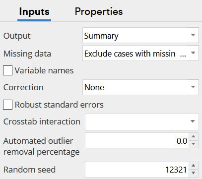
Below the warnings, you will find an option for setting the Automated outlier removal percentage. By default, this is set to 0. But, we can increase this percentage and remove the most outlying observations (based on studentized residuals for unweighted models and Pearson residuals for weighted models).
There is no magical rule for determining the optimal percentage to remove (if there was we would have automated it). Instead, you need to make judgments, trading off the following:
- The more observations you remove, the less the model represents the entire dataset. So, start by removing a small percentage (e.g., 1%).
- Does the warning disappear? If you can remove, say 10% of the observations and the warning disappears, that may be a good thing. But, it is possible that you always get warnings. It’s important to appreciate that the warnings are designed to alert to situations where rogue observations are potentially causing a detectable change in conclusions. But, often this change can be so small to be trivial.
- How much do the key conclusions change? If they do change a lot, you need to consider inspecting the raw data and working out why the observations are rogue (i.e., is there a data integrity issue?).
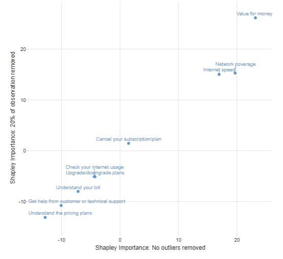
As an example, the scatterplot below shows the importance scores estimated for two Shapley Regressions, one based on the entire data set, and another based on 20% of observations being removed. With both regressions there are warnings regarding influential observations. However, we can see that while there are differences between the conclusions of the models (the estimated importance scores would be in a perfectly straight line otherwise), the differences are, in the overall scheme of things trivial and irrelevant, giving us some confidence that we can ignore the outliers and use the model without any outlier removal.