Using Hierarchical Bayes for MaxDiff in Displayr

Try your own MaxDiff Hierarchical Bayes

Getting started

Your MaxDiff data needs to be in the same format as the technology companies dataset used in previous blog posts on MaxDiff such as this one. To start a new Hierarchical Bayes analysis, click Insert > More > Marketing > MaxDiff > Hierarchical Bayes. Many options in the object inspector on the right are identical to those of latent class analysis and I shall not explain them here. Separate sections below describe the remaining options specific to Hierarchical Bayes.

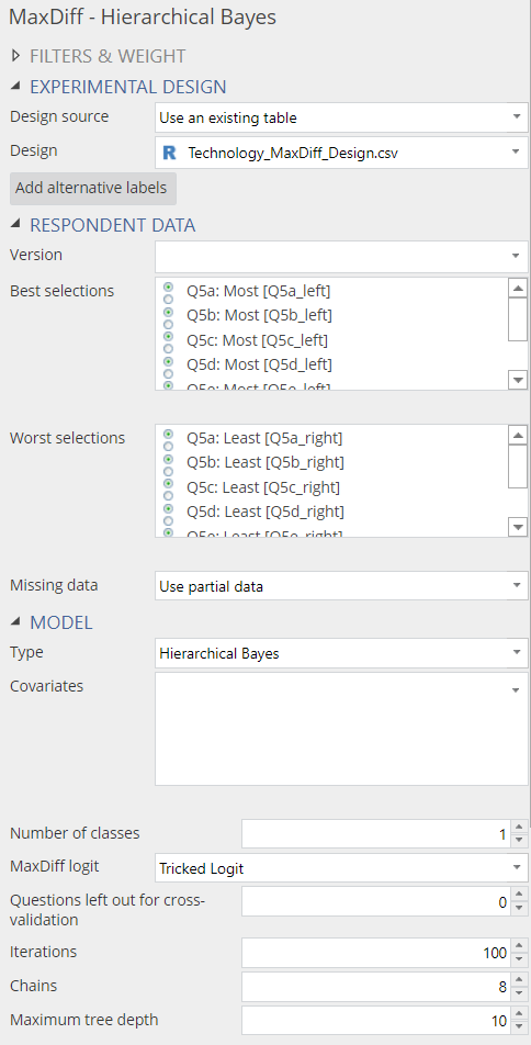
Number of Classes

This parameter controls the complexity of the model. If the data set contains discrete people, these segments may be missed if the number of classes is set to 1. A more complex model, which is one with more classes, is more flexible but takes longer to fit and may not necessarily provide better performance. If investigating more than one class, it is advisable to ensure it has better predictive accuracy than the one class solution (via cross-validation, discussed below).

If comparing results with Sawtooth, set this to 1: the number used in all Sawtooth models.

Try your own MaxDiff Hierarchical Bayes

Iterations

This option controls how long the analysis runs for. More iterations result in a longer computation time but often leads to better results.  When using fewer iterations, the possibility exists that the model returns premature results. In addition, warning messages may appear about divergent transitions or that the Bayesian Fraction of Missing Information is low. However, the absence of warning messages does not mean that the number of iterations is sufficient. I discuss this in more detail below.

Chains

This option specifies how many separate chains (independent analyses) to run, where the chains run in parallel, given the availability of multiple cores. Increasing the number of chains increases the quality of the results. It does, however, result in a longer running time if chains are queued up. Therefore I suggest leaving the option at its default value of eight.  This makes full use of the 8 cores available when running R code in Dispalyr.

Maximum tree depth

This is a very technical option, and I am not even going to try and explain it. The practical implication is that this option should only need to be changed if a warning appears indicating that the maximum tree depth has been exceeded. The default value is 10 and a warning should not appear under most circumstances. If such a warning does appear, I suggest first increasing the maximum tree depth to 12 rather than a larger number, as this could increase computation time significantly.

Download our free MaxDiff ebook

Output

The output of Hierarchical Bayes is a table with histograms showing the distribution of respondent coefficients. In the next few sections I describe other types of outputs created from the Insert > More > Marketing > MaxDiff > Diagnostic menu. The coefficients are scaled to have a mean of 0 across brands (i.e., the brand with the highest mean, in this case, Apple, is the most preferred brand). We can also see that some people like it less than average (which is shown by the proportion of the histogram in red). Apple is the most divisive brand, resulting in a wide range of coefficients. In contrast, a majority of respondents have a mildly positive view of Google and not many dislike it.

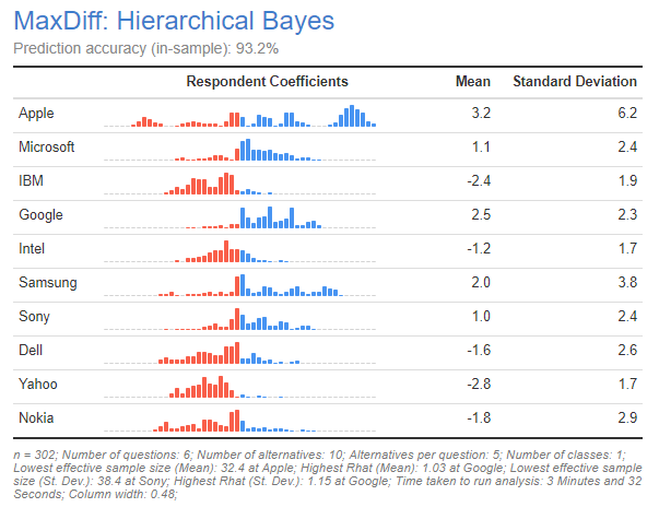
In addition to the distribution and mean value of the parameters, take note of the Prediction accuracy shown at the top of the output. This shows the percentage of questions in which the model correctly predicts the choice of most preferred. A number of different factors determine predictive accuracy:

• The consistency within the data. If people have given near-random data, then prediction accuracy will always be poor.
• The amount of data per person. The more data each person has provided, the higher the prediction accuracy, all else being equal.
• The number of iterations. If you have too few iterations, you will get poor predictive accuracy. You check this by checking convergence, further discussed below.
• Whether the predictions are in the sample or from cross-validation (as specified with the Questions left out for cross-validation control). Cross-validation predictive accuracy is typically considerably lower than in-sample accuracy.

Trace plots

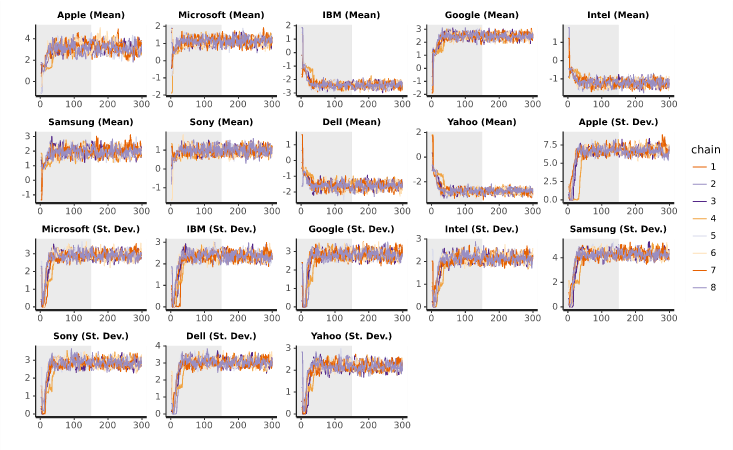
The plots below can be created by selecting a Hierarchical Bayes output and clicking on Insert > More > Marketing > MaxDiff  > Diagnostic > Trace Plots. The plots show how the main parameters change as the analysis progresses over the iterations for each chain. The grey half-section indicates the warm-up iterations, which are excluded from the final results. The non-grey part is the final result. With more than a couple of cores, these plots can be hard to read. Beyond the warm-up stage, the range of each chain should overlap almost entirely with those of the other chains. If one chain appears higher or lower than the others, this would indicate a problem with the model and more iterations may be required.

Posterior Intervals

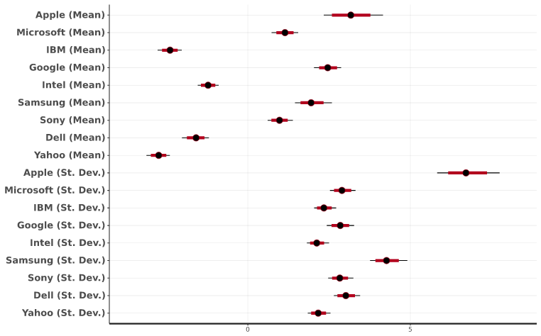
You create this plot by selecting a Hierarchical Bayes output and clicking on Insert > More > Marketing > MaxDiff  > Diagnostic > Posterior Intervals. This plot shows the range of the main parameters in the analysis. The black dot corresponds to the median, while the red line represents the 80% interval of the draws, and the thin black line is the 95% interval. The plot includes the distributions of the estimated means and standard deviations. This gives us an understanding of the uncertainty regarding conclusions shown in the earlier histograms. For example, comparing Apple and Google, we can see that there is little overlap in the distributions of the means, which tells us that the data shows a clear average preference for Apple being greater than for Google. Looking at the standard deviations, we can see that the value for Apple is, by far, the largest for any of the brands. This tells us that it is a divisive brand (i..e, some people love it, others like it much less), as we have observed earlier.

Parameter statistics

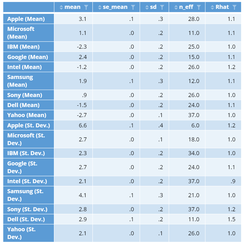
You can create this table by selecting a Hierarchical Bayes output and clicking on Insert > More > Marketing > MaxDiff  > Diagnostic > Parameter Statistics. The table output shows:

• the mean
• the standard error of the mean
• standard deviation
• the effective sample size, and
• the potential scale reduction statistic of the main parameters

What we want to see, are values of 100 or more in the n_eff column and ideally 1.1 or less in the Rhat column. Consequently, we can see problems with convergence for most of the standard deviation parameters in the below table. We need to re-run the model with more iterations until we fix these problems. I typically keep doubling the number of iterations until the problems go away. More detail about checking for convergence is in Checking Convergence When Using Hierarchical Bayes for MaxDiff.

Try your own MaxDiff Hierarchical Bayes

Using Hierarchical Bayes results in other analyses

Typically, once convergence has been established, the preferences for each respondent need to be extracted from the model and used in further analysis. The most straightforward approach to doing this is to select the model output (i.e., which shows the histograms and predictive accuracy), and select Insert > More > Marketing > MaxDiff > Save Variable(s) > Individual-Level Coefficients. This creates:

• One new variable for each of the alternatives. This is the raw data that is plotted as histograms in the standard output.
• A summary table showing the averages.

Individual-level coefficients can be difficult to interpret, as the scale is in logit-space. The most straightforward solution is to instead compute preference shares, which show, for each person, their probability of choosing each of the alternatives first:  Insert > More > Marketing > MaxDiff > Save Variable(s) > Compute Preference Shares.

For more advanced analyses, such as preference simulations, it can be useful to extract the posterior draws. These are individual-level coefficients, where there are multiple coefficients for each person. These estimates reflect the uncertainty of the estimated preferences. To do this, select the output that contains your model and then go to Properties > R CODE and modify the R code to add the following optional parameter hb.beta.draws.to.keep = 100 to the function call of FitMaxDiff (this parameter sets the number of samples per respondent to keep, which I have chosen to be 100 in this case). To obtain the posterior draws, create a new R Output (Insert > R Output), and enter the following code, replacing max.diff with the name of the model output (which may be max.diff, if you have only created one MaxDiff analysis):

max.diff$beta.draws[, 1, ]

This returns a matrix of the draws of the first respondent. With the row and column dimensions corresponding to the iterations and variables respectively. Iterations from the multiple chains make up the iterations dimension, with the warm-up iterations excluded. To get the draws from another respondent, simply change the 1 in the code with the respondent's index.