How to do Logistic Regression in Displayr

This is a practical guide to logistic regression. To get the most out of this post, I recommend you follow along with my instructions and do your own logistic regression. If you're new to Displayr, click the button below and add a new document!

Get started

Step 1: Importing the data

We start by clicking the  + Add a data set  button in the the bottom-left of the screen in Displayr and choosing our data source. In this example I am using a data set available on IBM's website, so we need to:

• Select the URL option.
• Paste in the following as the URL (web address): https://community.watsonanalytics.com/wp-content/uploads/2015/03/WA_Fn-UseC_-Telco-Customer-Churn.csv
• Set the automatic refresh to 999999 (to stop the data being re-imported and the model being automatically revised).

Step 2: Preliminary data checking

In order to build a logistic regression we need to decide which predictor variables (aka features) we wish to use in the model. This is a whole topic in itself, which I am going to side step in this post, by asserting that the predictors we want to use are the ones called SeniorCitizen, tenure, InternetService, Contract, and MonthlyCharge. The outcome variable to be predicted is called Churn. To perform a preliminary check of this data, hold down the control key and click on each of these variables (you should see them in the Data Sets, at the bottom-left of the screen - see below). Once they are selected, drag them (as a group) onto the page. Your screen should now look like this:

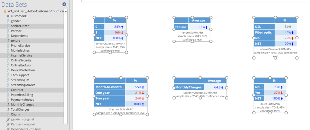
The specifics of how to perform a preliminary check of the data depend very much on the data set and problem being studied. In this section I am going to list what I have done for this case study and make some general comments, but please keep in mind that different steps may be required for your own data set. If you have any specific things you aren't sure about, please reach out to me and I will do what I can.

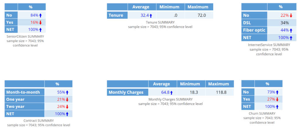
• The outcome variable, shown at the bottom-right, contains two categories, No and Yes. As (binary) logistic regression is appropriate with two categories, all is in order with this variable.
• Looking at the footer of the table, if you squint you will see that it shows a sample size of 7,043. Further, it mentions nothing about missing data (if there was missing data, it would be indicated in this footer). Looking at the other five tables, we can see that none have missing data, so all is good. If we had missing data we would have to make some enquiries as to its cause.
• The first of the tables, for the SeniorCitizen variable, shows values of 0 and 1 as the row names. In this case a 1 means the person is a senior citizen, and a 0 means that they are not. To make the resulting analysis a bit neater I:
  • Clicked on the SeniorCitizen variable in the Data Sets tree.
  • Changed its label to Senior Citizen (i.e., added a space) under GENERAL > Label in the Object Inspector.
  • Pressed the DATA VALUES > Labels button in the Object Inspector and changed the 0 to No and the 1 to Yes in the Label column and pressed OK. The table will automatically update to show the changes we have made to the the underlying data.
• Clicked on the variable table showing tenure and changed the variable's label to Tenure (i.e., making the capitalization consistent with the rest of the variables, so that the resulting outputs are neat enough to be shared with stakeholders).
• Changed MonthlyCharges to Monthly Charges.
• Changed InternetService to Internet Service.
• Clicked on the No category in the Internet Service table and clicked on the three grey lines that appear to its right (if you don't see them, click again), and dragged this category to be above DSL. If you accidentally merge the categories, just click the Undo arrow at the top-left of the screen. (Making sure that the categories are ordered sensibly makes interpretation easier.)
• Selected the Tenure and Monthly Charges tables, and then, in the Object Inspector, clicked Statistics > Cells and clicked on Maximum and then Minimum, which adds these statistics to the table. In order to read them, click on the two tables that are on top, and drag them to the right so that they do not overlap. The good thing to note about both of these tables is that the averages, minimum, and maximum all look sensible, so there is no need to do any further data checking or cleaning.

If all has gone well, your screen should show the following tables.

Step 3: Creating an estimation, validation, and testing samples

What is described in this stage is best practice. If you have a small sample (e.g., less than 200 cases) or are doing your work in an area where model quality is not a key concern, you can perhaps skip this step. However, before doing so, please read Feature Engineering for Categorical Variables, as it contains some good examples illustrating the importance of using a validation sample.

In order to check our model we want to split the sample into three groups. One group will be used for estimating our model. This group of data is referred to as the estimation or training sample. A second group is used when comparing different models, which is called the validation sample. A third group is used for a final assessment of the quality of the model. This is called the test or testing sample. Why do we need these three groups? A basic problem when building predictive models is overfitting, whereby we inadvertently create a model that is really good at making predictions in the data set used to create the model, but which performs poorly in other contexts. By splitting the data into these three groups we can partly avoid overfitting, as well as assess the extent to which we have overfit our model.

In Displayr, we can automatically create filters for these three groups using Insert  > Utilities (More) > Filtering > Filters for Train-Validation-Test Split, which adds three new variables to the top of the data set, each of which has been tagged as Usable as a filter. The first of the filters is a random selection of 50% of the sample and the next two have 25% each. You can modify the proportions by clicking on the variables and changing the value in the first line of the R CODE for the variable.

Step 4: Creating a preliminary model

Now we are ready to build the logistic regression:

• Insert > Regression > Binary Logit (binary logit is another name for logistic regression).
• In Outcome select Churn.
• In Predictor(s) select Senior Citizen, Tenure, Internet Service, Contract, and Monthly Charge. The fastest way to do this is to select them all in the data tree and drag them into the Predictor(s) box.
• Scroll down to the bottom of the Inputs tab in the Object Inspector and set FILTERS & WEIGHTS > Filter(s) to Training sample.
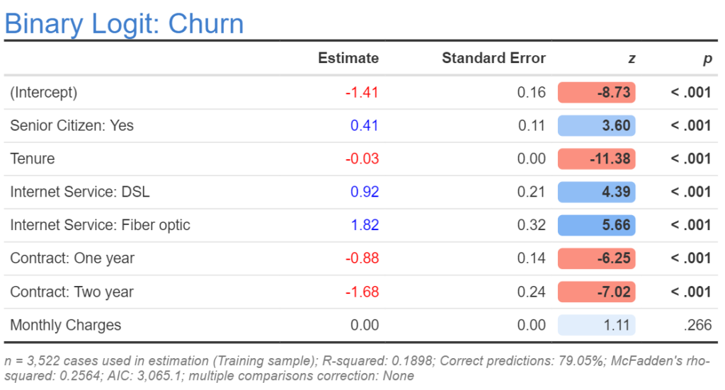
• Press Automatic, which ensures that your model updates whenever you modify any of the inputs. If all has gone to plan, your output will look like this:

Step 5: Compute the prediction accuracy tables

• In Displayr, click on the model output (which should look like the table above).
• Insert > Regression > Diagnostic > Prediction-Accuracy Table.
• Move this below the table of coefficients and resize it to fit half the width of the screen (alternatively, add a new page and drag it to this page).
• Making sure you still have the prediction-accuracy table selected, click on Object Inspector > Inputs > Filter(s) and set it to Training sample, which causes the calculation only to be based on the training sample. The accuracy (shown in the footer) should be 79.05% as in the table above.
• Press Home > Duplicate (Selection), drag the new copy of the table to the right, and change the filter to Validation sample. This new table shows the predictive accuracy based on the validation sample (i.e., the out-of-sample prediction accuracy). The result is almost the same, 79.1%.

Step 6: Interpretation

Nice work! You have created all the key outputs required for logistic regression. For details on how to read them, please see How to Interpret Logistic Regression Coefficients and How to Interpret Logistic Regression Outputs.

Step 7: Modeling checking, feature selection, and feature engineering

The next step is to tweak the model, by following up on any warnings that are shown, and by adding, removing, and modifying the predictor variables. See Feature Engineering in Displayr and Feature Engineering in Displayr for more information.

If you want to look at the various analyses discussed in this post in more detail, click here to get a copy of the Displayr document that contains all the work. Alternatively, reproduce the analyses yourself (downloading the data in Step 1) or use your own data.

Do your own logistic regression in Displayr!