

This post describes how to interpret the coefficients, also known as parameter estimates, from logistic regression (aka binary logit and binary logistic regression). It does so using a simple worked example looking at the predictors of whether or not customers of a telecommunications company canceled their subscriptions (whether they churned).
If you're new to regression analysis, you might find it helpful to start with linear regression, which lays the foundation for understanding more complex models like logistic regression.
The case study: customer switching
The table below shows the main outputs from the logistic regression. No matter which software you use to perform the analysis you will get the same basic results, although the name of the column changes. In R, SAS, and Displayr, the coefficients appear in the column called Estimate, in Stata the column is labeled as Coefficient, in SPSS it is called simply B. The output below was created in Displayr. The goal of this post is to describe the meaning of the Estimate column.
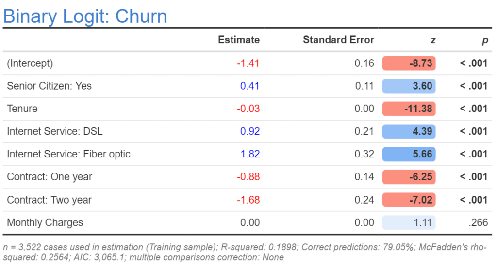
Although the table contains eight rows, the estimates are from a model that contains five predictor variables. There are two different reasons why the number of predictors differs from the number of estimates. The estimate of the (Intercept) is unrelated to the number of predictors; it is discussed again towards the end of the post. The second reason is that sometimes categorical predictors are represented by multiple coefficients. The five predictor variables (aka features) are:
- Whether or not somebody is a senior citizen. This is a categorical variable with two levels: No and Yes. Note that in the output below we can only see Yes. The reason for this is described below.
- How long somebody had been a customer, measured in the months (Tenure). This is a numeric variable, which is to say that the data can in theory contain any number. In this example, the numbers are whole numbers from 0 through to 72 months. We can see from the output that this is a numeric predictor variable because no level names are shown after a colon.
- Their type of Internet Service: None, DSL, or Fiber optic. (Again, None is not shown.)
- Contract length: Month-to-month, One Year, or Two years. (Again, Month-to-month is not shown.)
- Monthly Charges, in dollars. This is also a numeric variable.
Create your own logistic regression
The order of the categories of the outcome variable
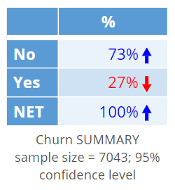
To interpret the coefficients, we need to know the order of the two categories in the outcome variable. The most straightforward way to do this is to create a table of the outcome variable, which I have done below. As the second of the categories is the Yes category, this tells us that the coefficients above are predicting whether or not somebody has a Yes recorded (i.e., that they churned). If the table instead showed Yes above No, it would mean that the model was predicting whether or not somebody did not cancel their subscription.
Create your own logistic regression
The signs of the logistic regression coefficients
Below, I have repeated the table to reduce the amount of time you need to spend scrolling when reading this post. As discussed, the goal in this post is to interpret the Estimate column and we will initially ignore the (Intercept). The second Estimate is for Senior Citizen: Yes. The estimate of the coefficient is 0.41. As this is a positive number, we say that its sign is positive (sign is just the jargon for whether the number is positive or negative). A positive sign means that all else being equal, senior citizens were more likely to have churned than non-senior citizens. Note that no estimate is shown for the non-senior citizens; this is because they are necessarily the other side of the same coin. If senior citizens are more likely to churn, then non-senior citizens must be less likely to churn to the same degree, so there is no need to have a coefficient showing this. The way that this "two-sides of the same coin" phenomena is typically addressed in logistic regression is that an estimate of 0 is assigned automatically for the first category of any categorical variable, and the model only estimates coefficients for the remaining categories of that variable.
Now look at the estimate for Tenure. It is negative. As this is a numeric variable, the interpretation is that all else being equal, customers with longer tenure are less likely to have churned.
The Internet Service coefficients tell us that people with DSL or Fiber optic connections are more likely to have churned than the people with no connection. As with the senior citizen variable, the first category, which is people not having internet service, is not shown, and is defined as having an estimate of 0.
People with one or two year Contracts were less likely to have switched, as shown by their negative signs.
In the case of Monthly Charges, the estimated coefficient is 0.00, so it seems to be unrelated to churn. However, we can see by the z column, which must always have the same sign as the Estimate column, that if we showed more decimals we would see a positive sign. Thus, if anything, it has a positive effect (i.e., more monthly charges leads to more churn).
Create your own logistic regression
The magnitude of the coefficients
We can also compare coefficients in terms of their magnitudes. In the case of the coefficients for the categorical variables, we need to compare the differences between categories. As mentioned, the first category (not shown) has a coefficient of 0. So, if we can say, for example, that:
- The effect of having a DSL service versus having no DSL service (0.92 - 0 = 0.92) is a little more than twice as big in terms of leading to churn as is the effect of being a senior citizen (0.41).
- The effect of having a Fiber optic service is approximately twice as big as having a DSL service.
- If somebody has a One year contract and a DSL service, these two effects almost completely cancel each other out.
Things are marginally more complicated for the numeric predictor variables. A coefficient for a predictor variable shows the effect of a one unit change in the predictor variable. The coefficient for Tenure is -0.03. If the tenure is 0 months, then the effect is 0.03 * 0 = 0. For a 10 month tenure, the effect is 0.3 . The longest tenure observed in this data set is 72 months and the shortest tenure is 0 months, so the maximum possible effect for tenure is -0.03 * 72= -2.16, and thus the most extreme possible effect for tenure is greater than the effect for any of the other variables.
Returning now to Monthly Charges, the estimate is shown as 0.00. It is possible to have a coefficient that seems to be small when we look at the absolute magnitude, but which in reality has a strong effect. This can occur if the predictor variable has a very large range. In the case of this model, it is true that the monthly charges have a large range, as they vary from $18.80 to $8,684.40, so even a very small coefficient (e.g., 0.004) can multiply out to have a large effect (i.e., 0.004 * 8684.40 =34.7). However, as the value is not significant (see How to Interpret Logistic Regression Outputs), it is appropriate to treat it as being 0, unless we have a strong reason to believe otherwise.
Create your own logistic regression
Predicting probabilities
We can make predictions from the estimates. We do this by computing the effects for all of the predictors for a particular scenario, adding them up, and applying a logistic transformation.
Consider the scenario of a senior citizen with a 2-month tenure, with no internet service, a one-year contract, and a monthly charge of $100. If we compute all the effects and add them up we have 0.41 (Senior Citizen = Yes) - 0.06 (2*-0.03; tenure) + 0 (no internet service) - 0.88 (one year contract) + 0 (100*0; monthly charge) = -0.53.
We then need to add the (Intercept), also sometimes called the constant, which gives us -0.53- 1.41 = -1.94. To make the next bit a little more transparent, I am going to substitute -1.94 with x. The logistic transformation is:
Probability = 1 / (1 + exp(-x)) = 1 /(1 + exp(- -1.94)) = 1 /(1 + exp(1.94)) = 0.13 = 13%.
Thus, the senior citizen with a 2 month tenure, no internet service, a one year contract, and a monthly charge of $100, is predicted as having a 13% chance of cancelling their subscription. By contrast if we redo this, just changing one thing, which is substituting the effect for no internet service (0) with that for a fiber optic connection (1.86), we compute that they have a 48% chance of cancelling.
Create your own logistic regression
Transformed variables
Sometimes variables are transformed prior to being used in a model. For example, sometimes the log of a variable is used instead of its original values. Very high values may be reduced (capping). Predictors may be modified to have a mean of 0 and a standard deviation of 1. Effects coding may have been used with categorical variables (which means that the first category may have a value of -1 rather than 0). When variables have been transformed, we need to know the precise detail of the transformation in order to correctly interpret the coefficients.
Create your own logistic regression
Odds ratios
In some areas it is common to use odds rather than probabilities when thinking about risk (e.g., gambling, medical statistics). If you are working in one of these areas, it is often necessary to interpret and present coefficients as odds ratios. If you are not in one of these areas, there is no need to read the rest of this post, as the concept of odds ratios is of sociological rather than logical importance (i.e., using odds ratios is not particularly useful except when communicating with people that require them).
To understand odds ratios we first need a definition of odds, which is the ratio of the probabilities of two mutually exclusive outcomes. Consider our prediction of the probability of churn of 13% from the earlier section on probabilities. As the probability of churn is 13%, the probability of non-churn is 100% - 13% = 87%, and thus the odds are 13% versus 87%. Dividing both sides by 87% gives us 0.15 versus 1, which we can just write as 0.15. So, the odds of 0.15 is just a different way of saying a probability of churn of 13%.
Consider now the second scenario, where we found that replacing no internet connection with a fiber optic connection caused the probability to grow to 47% which, expressed as odds, is 0.89.
We can compute the ratio of these two odds, which is called the odds ratio, as 0.89/0.15 = 6.
Earlier, we saw that the coefficient for Internet Service:Fiber optic was 1.82. A shortcut for computing the odds ratio is exp(1.82), which is also equal to 6. So, if we need to compute odds ratios, we can save some time. (If you reproduce this example you will get some discrepancies, caused by rounding errors.)
Now that you've learnt how to interpret logistic regression coefficients, you can quickly create your own logistic regression in Displayr.
Sign up for free