The difference between a numeric and categorical price attribute
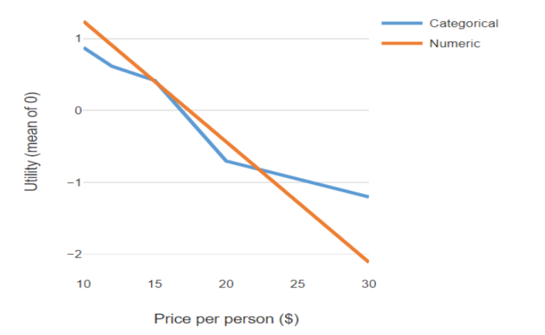
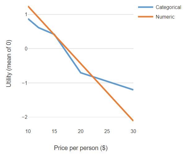
The chart below illustrates the the implications of treating price as being categorical versus numeric. When price is treated as a numeric attribute (variable), the model assumes that there is a linear relationship between price and utility, as shown by the orange line. When price is modeled as being categorical, non-linear relationships can be found. In this example, which is from the home deliver market, the categorical price attribute leads to the conclusion the drop in utility that goes with changing price from $15 to $20 is particularly large, being much larger than the drop from $10 to $15 and even from $20 to $30. By contrast, when a numeric price attribute is used, the model assumes that the effect is constant across all price points; each extra dollar of price leads to a constant drop off in utility.
The benefit of treating price as being categorical
The key benefit of treating price as being categorical is that it is more consistent with what we know about consumer behavior. Study after study has found interesting non-linear relationships between price and consumer preferences, and in marketing it is the norm to view these as indicating interesting “psychological” pricing findings. For example, in most markets there are believed to be price thresholds (e.g., keep a phone under $1,000), and various other interesting pricing points (e.g., prices ending in 99). Identifying such psychological price points and using them as a basis for setting price seems like good strategy.
The benefits of treating price as numeric
Economic theory suggests that the relationship between price and utility should be linear. To use the jargon: the price coefficient is seen as being the marginal utility of income. Although it is routine for studies to find statistical evidence that the price is nonlinear, it is possible that psychological price points are just research artifacts. Perhaps surveys show non-linearity, but in the real world with real money people behave more rationally.
When we treat price as being a numeric attribute, it allows us to use interpolation and extrapolation to make more precise conclusions about price. In the example above, where we have treated price as being categorical, we can only safely draw conclusions at the specific price points tested in the research. In this case, these are $10, $12, $15, $20, and $30 (i.e., the end-points and the places where the lines join). By contrast, with the numeric variable we can price at any point along the line, and if we are brave can extrapolate beyond the line. Further, with the numeric attribute the effect of sampling error is smaller so we can have even more confidence about our conclusions.
Another benefit of treating price as being numeric is that it allows you to use choice modeling with data that has too many different price points to make it practical to estimate a separate utility for each price point. Such data is widespread in economics and transportation researcher, where the prices that are shown to each respondent are customized to their specific circumstances (e.g., if an attribute is the price of traveling by car, each person’s fuel costs and depreciation will be slightly different).
There is a further benefit of treating price as being numeric: it makes it a lot simpler to make price-related conclusions from the research. The next section provides a bit more detail on how to interpret price effects estimates when price is treated as being numeric. Then, I discuss how this simplifies other calculations.
How to interpret numeric price coefficients
The output below shows the estimated distribution of a numeric attribute relating to price of home delivered food. It would be very easy to look at this and conclude that, relative to Cuisine, Price per person is both not very important and that there is very little variation in terms of its importance in the population. However, this is not the right way to read this output.
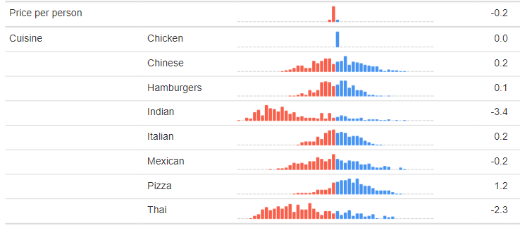
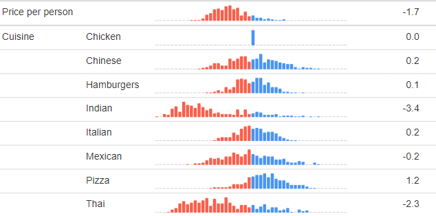
To illustrate this point, the output below shows a model that I have re-estimated, but rather than using prices of 10, 12, 15, 20, and 30, I’ve divided them by 10 and have used prices of 1, 1.2, 1.5, 2. and 3. Price appears to be much more important below, but in reality it is equally important in both models. The thing to keep in mind is that the values shown for Cuisine are utilities, whereas the distribution shown for Price per person is instead a coefficient. For categorical data the ideas of a utility and a coefficient are interchangeable, but with numeric attributes they are not. In order to compute utility, we need to multiply the coefficient of the numeric attribute by the values. In the output above, it shows that the coefficient for Price per person is 0.2; this is rounded, and with an extra decimal the value is -0.17. The utility for $10 is then 10*-.17 = -1.7 and the utility for $30 is 30*-.17 = -5.1.
Computing average willingness-to-pay
When we have a price coefficient, we can easily scale all other utilities by dividing by this coefficient. For example, where the coefficient for price is 0.17, using the data shown above, we end up computing the average mean utility for the different cuisines as follows:
- Chicken: $0
- Chinese: $1.18
- Hamburgers: $0.59
- Indian:-$20.00
- Italian: $1.18
- Mexican: $-$1.18
- Pizza:$7.06
- Thai: -$13.53
These are variously known as dollar-metric utilities and as willingness-to-pay (WTP). Comparing, for example, Chinese with Hamburgers, Chinese has a $0.59 higher WTP ($1.18 – $0.59), and an interpretation of this is that, on average, people are prepared to pay $0.59 more for a Chinese meal than a hamburger meal.
There are a series of posts that provide more details about different aspects of numeric attributes in choice models:
- Testing Whether an Attribute Should be Numeric or Categorical in Conjoint Analysis
- Numeric Attributes in Conjoint Analysis in Displayr
- Using Utilities Plots to Facilitate Comparison of Numeric and Categorical Attributes in Conjoint Analysis.
- Using Conjoint Analysis to Set Prices describes more
You can view these calculations, hooked up to the raw data and models in Displayr, by clicking here.
The easiest way to avoid any possibility of misunderstanding is to use Insert > Conjoint/Choice Modeling > Utilities Plot, which automatically computes the utility for the highest and lowest prices in the study.