


A simulation involving two segments
To explore this problem I generated some simulated data for 200 fake respondents. I used a MaxDiff experiment with 10 alternatives (A, B, …, J) and 2 segments (75% and 25% in size). One segment was created to prefer the alternatives in order of A > B > … > J with coefficients of 4.5, 3.5., …, -4.5. The second segment had the coefficients in the reverse order.
The models
I estimated six models:
- A multinomial logit model (using Tricked Logit for this and all models, to deal with the worst choices).
- A latent class logit model with 2 classes (i.e., latent class analysis with multinomial logit estimated in each class).
- A latent class logit model with 3 classes.
- A standard HB model.
- A 2-class HB model. This is a hybrid of latent class analysis and HB, where the model assumes that the data contains two segments, where each segment has its own HB model.
- A 3-class HB model.
Predictive accuracy of the models
The experimental design contained 6 questions with 5 options in each. I used 4 of the questions, randomly selected for each respondent, to fit the models, using the remaining 2 for cross-validation purposes. The predictive accuracy from the cross-validation is shown below. In most regards these results are as we would expect. The latent class logit with 2 classes outperforms the standard HB model. So does the 2-class HB model. Both three class models perform the same. The one result that was really surprising to me is that the standard HB model does surprisingly well.
| Number of classes | Latent Class Analysis | Hierarchical Bayes |
|---|---|---|
| 1 | 62.3% | 78.5% |
| 2 | 82.0% | 82.0% |
| 3 | 82.0% | 82.0% |
Investigating the standard HB model
To better understand the performance of the standard HB model I computed the individual-level coefficients and formed them into two segments using K-means cluster analysis. It perfectly recovered the two segments – that is, each person was classified into the correct segment. This is obviously very good news, as it suggests that from the perspective of forming segments, we can achieve this result with HB, even when latent class analysis is the theoretically better model.
Nevertheless, the table above shows that the standard HB model (first row, last column) has worse predictive accuracy than latent class analysis (second row, second column). As mentioned above, I simulated the data with coefficients of -4.5, -3.5, -2.5, …, 4.5, and the reverse in the second segment. The chart below shows the estimated averages for each segment from the standard HB model. HB has correctly recovered the relative order of the preferences, but the average coefficients are incorrect. They are, by and large, more extreme. For example, alternative J is estimated as having a coefficient of 7.3 and -6.1, whereas the correct values are -4.5 and 4.5. (By contrast, the values estimated for the latent class analysis, which are not shown, were almost identical to the simulated values, as we would expect given that the data was generated under the assumption of latent classes).
A second problem emerges when when we look at the distributions of the individual-level coefficients. Below, to the left, I have shown density plots of the distributions from the latent class analysis for people in the first segment. On the right I show the distributions as estimated from the standard HB for the same respondents. In addition to the means being further from 0, the HB is estimating a lot of variation within the segments, and this is largely incorrect. For example, for alternative A, shown at the bottom, the latent class analysis estimates a value of -4.4 relative to the true value of -4.5, whereas the HB model incorrectly indicates that there is variation within the segment from around -11 to 0, with a median of about -7.
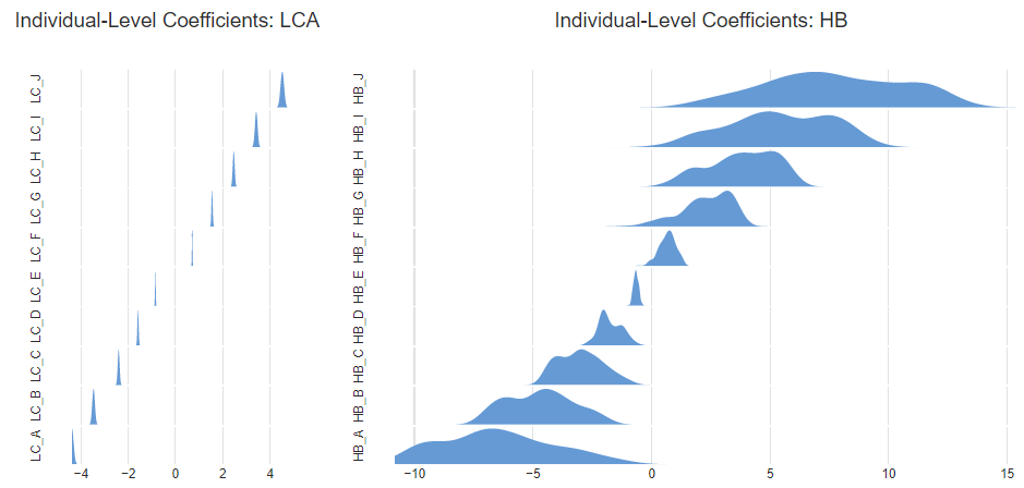
If the only focus is creating segments, this difference is pretty trivial in this example, but this would not always be the case. If the individual-level coefficients are used for other purposes, such as correlating with other data or computing preference shares, these errors become more important.
Multi-class HB is better
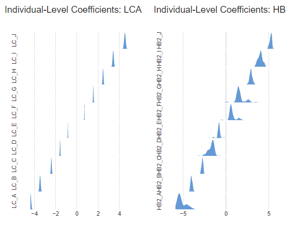
As shown earlier, the 2 and 3-class HB models had the same predictive accuracy as the 2-class Latent Class model. The chart compares the estimated individual-level coefficients with those from the Latent Class Analysis. The 2-class HB model is not quite as good as the Latent Class Analysis model, but the differences are small (particularly compared to the standard HB).
Implications
The simulation that I describe in this post shows that if the data does contain segments, latent class analysis will do a better job than the one-class HB models that most MaxDiff practitioners use. This supports the conventional wisdom about the different strengths of these models. However, in real-world situations we do not always know whether the data truly contains segments. As a result, the best strategy is generally to compare multiple models based on predictive accuracy. The best model in general seems likely to be an HB model with multiple classes, as this has the flexibility to be useful regardless of whether segmentation exists or not.
See how we conducted this analysis in Displayr, or to find out more, head to the visualization page of our blog!