The Correct Treatment of Sampling Weights in Statistical Tests

Case study

A simple case study is used to illustrate the issue. It contains two categorical variables, one measuring favorite cola brand (Pepsi Max vs Other), and the other measuring gender. The data set contains five weights, each of which is used to illustrate a different aspect of the problem. The data is below. All the calculations illustrated in this post are in this Displayr document.

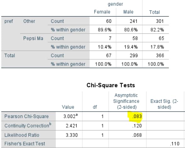
Consider first an analysis that doesn't use any of the weight variables (an unweighted analysis). The output below shows a crosstab created in SPSS. A few key points to note:

• For the purposes of this post, it is easiest to think of this test as comparing the proportions of Females that prefer Pepsi Max (10.4%) with the proportion of Males (19.4%).
• The sample sizes are 67 Female and 299 for Male, respectively.
• The standard chi-square test results are shown in the Pearson Chi-Square row of the Chi-square tests table and it's p-value is .083. So, if using the 0.05 cutoff we would conclude there is no relationship between Pepsi Max and gender.
• Four other tests are shown on the table. Pearson's tests is probably the best for this table (for reasons beyond the scope of this post). However, the other tests, which make slightly different assumptions are giving broadly similar results. This point's important: different tests with different assumptions will give different, but similar, results, provided the assumptions aren't inappropriate.

If you studied statistics, there's a good chance you were taught to do a Z-test to compare the two proportions. The calculations below perform this test. They are written in the R language, but if you take the time you will find it easy to follow the calculations. The computation of the statistic is different from the chi-square test statistic but the tests are equivalent in this unweighted case with identical p-values.

Getting the wrong answer using weights in SPSS

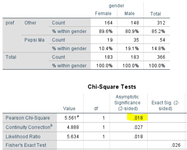
The output below shows the SPSS results with a weight (wgt1) applied.  These results are incorrect for two reasons. The first reason is that, by default, SPSS has rounded the cell counts, and used these rounded cell counts in the chi-square test and the percentages, meaning that every single number in the analysis is, to a small extent, wrong. (In fairness to SPSS, this routine was presumably written in the mid-1960s, and this type of hack may have been necessary for computational reasons back then.)

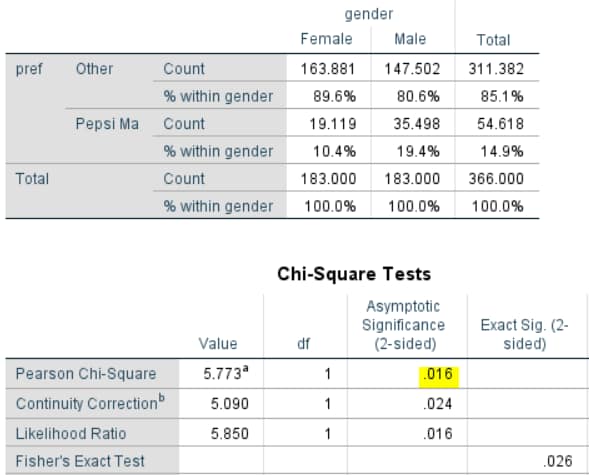
The output below uses the un-rounded results. The first thing to note is that that the p-value is much lower than with the unweighted result (.016 versus .08). If testing at the .05 level, you would conclude the difference is significant. So, you may end up with a completely different conclusion. Which, if either, is correct? In this case, the unweighted result is correct. Let me explain:

• If you look at the table below, you will see that it reports the same percentages as in the earlier example: 10.4% for Female and 19.4% for Male. So, the weights have not changed the results at all. Why? We weight data to correct for over- and under-representation in a sample. In this example, the weight is correcting for an under-representation of women. Consequently, the weight does not change the percentages in any way, as the percentages are within the gender groups.
• Note that the sample size for the Female group is shown in the table as 183 and the same sample size is shown for the male groups. And, this is how SPSS has computed the test. It has used the weighted sample size when conducting the test. This is obviously wrong. In the sample we only have 67 females. The weight doesn't change this. Whether we weight or not, we still only have data for 67 females, so performing a statistical test that assumes we have data from 183 females is not appropriate.
• This isn't really a flaw of SPSS. If you read its documentation it explains that it is not meant to be used with sampling weights. SPSS even a special module called Complex Samples which will perform the problem correctly and is what they recommend you use.

Getting the wrong answer using regression in R

The example above can't be reproduced in R, because its standard tools for comparing proportions don't even allow you to use weights of any kind. However, we can illustrate that the problem exists in routines in R that do support weights, such as regression.

Unweighted logistic regression

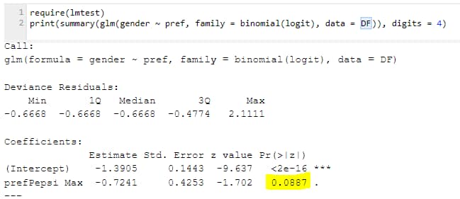
It's possible to redo the statistical test above using a logistic regression. This is illustrated below. The yellow highlighted number of 0.0887 is the p-value of interest. It's basically the same as we got with the standard chi-square test used at the beginning of the post (it had a p-value of .083). This statistical test in the logistic regression is assessing something technically slightly different and it's typical that tests that present slightly different technical answers get slightly different results.

Weighted logistic regression

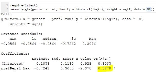
R's logistic regression does allow us to provide a weight. The output is shown below. Note that once again the p-value has gotten very small. The reason is that the weighted regression is, in its internals, making exactly the same mistake we saw with SPSS's chi-square test: it's assuming that the weighted sample size is the same thing as the actual sample size. Note that it basically gets the same result as with the chi-square test as well. So, we get the wrong answer by supplying a weight.

Doing the analysis properly

In the world of statistical theory, this is a solved problem. All of the techniques above correctly compute the percentages with the weights. More generally, all the parameters calculated using traditional statistical techniques, be they percentages, regression coefficients, cluster means, or pretty much anything else are typically computed correctly with weights. What goes wrong relates to the calculation of the standard errors. Below I reproduce the proportions test code shown earlier in the post. When the data is weighted, the lines of the code that are wrong are on lines 5-6. You can see based on first principles that it must be wrong, as it has no place to insert the weights. A correct solution is to rewrite lines 5-6, using a technique known as Taylor Series Linearization to calculate the standard error (se) in a way that addresses the weights appropriately. This is, sadly, not a trivial thing to do. I will disappoint you and not provide the math describing how it works, as the math will take a page, and, unless you have good math skills it's not a page that will help you at all. Last time I checked there were no good web pages about this topic. If you want to dig into how the math works, as well explore alternatives to Taylor Series Linearization, please read Chapter 9 of Sharon Lohr's (2019):  Sampling: Design and Analysis. But, warning, it's hard going.

So, how do we do the math properly? The secret is to use software designed for the problem. This means:

• Use our products: Q and Displayr. They get the right answer for problems like this by default.
• Use Stata. It provides excellent support for sampling weights (which it calls pweights).
• Use IBM SPSS Complex Samples. SPSS has a special module designed for weighted data. It will give you the correct results as well.
• Use the survey package in R

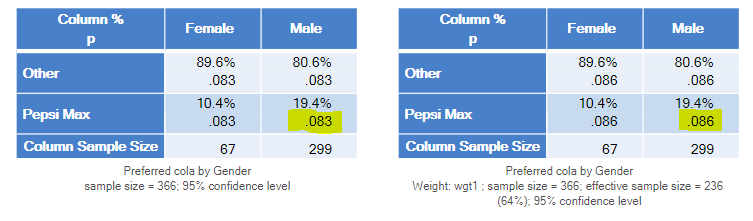
For example, the table below on the left shows the data in a Displayr crosstab that is unweighted. This gives the same result as we saw for the unweighted chi-square test in SPSS. The table on the right is using Taylor Series Linearization as a part of a test called the Second-Order Rao-Scott Chi-Square Test. It basically gets the same answer. That is, the Taylor Series Linearization gets the correct answer. You don't need to do anything special in Displayr and Q to have the Taylor Series Linearization applied; when you apply the weight it does this automatically.

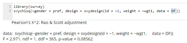
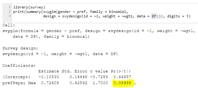
Similarly, here's the same calculation done using R:

The hacks (which don't work)

Most experienced survey researchers are familiar with these problems, and they typically employ one of four hacks as an attempt to fix the problem. These hacks are often better than ignoring the problem, but they are all inaccurate. In each case, they are attempts to limit the size of the mistakes that are made with using software not designed for sampling weights. None of the hacks solves the real problem, which is to validly compute the standard error(s).

Using the unweighted sample size

In the example above, we saw that the result was wrong because the weighted sample was used in the analysis, and this was clearly wrong. Further, in this example, we can compute the correct result using the weighted proportions and the unweighted sample size. However, this doesn't usually work. It only works in the example above because we were comparing percentages between the genders, and gender was the variable that was used in the weighting. It is easy to construct examples where using the unweighted sample size fails.

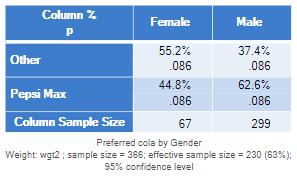
To appreciate the problem I re-run the same example, but using a different weight, wgt2,  which weights based on the row variable in the table. You will recall before that we have been comparing 10.4% with 19.1%. With the new weight, the percentages have changed dramatically, and we now have preferences for Pepsi Max of 44.8% and 62.6%. Note that the p-value in this example remains at .086.

However, when we compare the weighted proportions, but use the unweighted sample size, we get a very different result. Again, this incorrect analysis suggests a highly significant relationship, which is wrong.

Performing statistical testing without weights

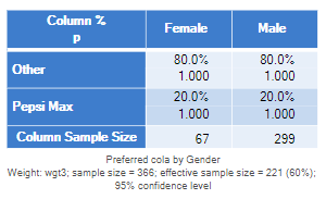
If you have been carefully reading through the above analyses, you will have realized that in each of the examples, the correct answer was obtained by performing the test using the unweighted data. However, this isn't generally a smart thing to do. The only reason that it works in the examples above is because we are testing two proportions and the weights are perfectly correlated with one of those variables in each of the tests above. It is easy to construct an example where using the unweighted data for testing gives the wrong answer. In the table below, after the weight has been applied (wgt3), there is no difference between the genders. As you would expect, the p-value, computed using the Taylor Series Linearization, is 1. However, the unweighted data still would show a p-value of .086, which is not sensible given there is no difference between the proportions.

Scaling weights to have an average of 1

When using statistical routines not designed for sampling weights, it is easy to get obviously wrong results in situations where the weights are large or small. In academic and government statistics it is common to create a weight that sums up to 1. When this is done, if using software that treats the weighted sample size as the actual sample size, nothing is ever shown as statistically significant. It is also common to creates weights that sum to the population size, as this means that all analyses are extrapolated to the population. This has the effect of making all analyses statistically significant. A common hack for both of these problems is to scale the weight to have an average value of 1. This is certainly better than using the unscaled weights, but it doesn't fix the problem. This has already been shown above, as all the calculations above have been performed using a weight with an average value of 1, and, as shown, the p-value was not computed correctly.

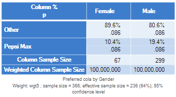
In addition to correctly computing the p-values, the useful thing about using routines designed for sampling weights, is that you don't need to rescale the weights at all. This means that you can use weights that gross up to the population size. In the table below, for example, which is from Displayr, the weighted sample size of each gender is 100,000,000, and the p-value is unchanged.

Using the effective sample size in calculations

The last of the hacks is to use Kish's effective sample size approximation when computing statistical significance. This is typically implemented in one of three ways:

• The weight is rescaled so that it sums to the effective sample size.
• The effective sample size is used instead of the actual sample size in the statistical test formulas.
• The effective sample size for sub-groups is used in place of the actual sample size for sub-groups in the statistical test formulas.

This hack is widespread in software. It is used in all stat tests in most of the older survey software packages (e.g., Quantum, Survey Reporter). We use it in some places in Q and Displayr, where the math for Taylor Series Linearization is intractable, inappropriate, or is yet to be derived. For example, there is no nice solution to dealing with weights when computing correlations, so we rescale the weights to the effective sample size.

This approach is typically better than any of the other hacks. But, it is still a hack and will almost always get a different (and thus wrong) answer to that obtained using Taylor Series Linearization. For example, below I've used the effective sample size for the first weight, and same (incorrect) result as obtained when using the unweighted sample size (they will not always coincide).

To summarize: if you have sampling weights you are best advised to use statistical routines specifically designed for sampling weights. Using software not designed for sampling weights leads to the wrong result, as do all the hacks.

All the non-SPSS calculations illustrated in this post are in this Displayr document.