5 Ways to Deal with Missing Data in Cluster Analysis

How to deal with missing data in cluster analysis

If you are not sure about cluster analysis or want to refresh your memory, check out our post on "What is cluster analysis" first. In this post I explain and compare the five main options for dealing with missing data when using cluster analysis:

• Complete case analysis
• Complete case analysis followed by nearest-neighbor assignment for partial data
• Partial data cluster analysis
• Replacing missing values or incomplete data with means
• Imputation

Missing data in cluster analysis example 

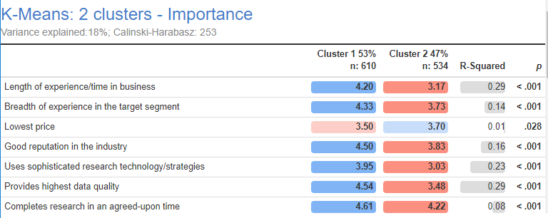
1,145 market research consultants were asked to rate, on a scale of 1 to 5, how important they believe their clients regard statements like Length of experience/time in business and Uses sophisticated research technology/strategies. Each consultant only rated 12 statements selected randomly from a bank of 25. Thus, each respondent has 13 missing values. Read on to discover the five ways of dealing with missing data in cluster analysis.

Complete case analysis

Performing clustering using only data that has no missing data forms the basic underlying idea of complete case analysis. In my example, no such data exists.  Because each consultant has 13 missing values, the cluster analysis fails.

Even if some data is available, complete case analysis is a pretty dangerous approach.  It is only valid when the cases with missing data have essentially the same characteristics as the cases with complete data. The formal statistical jargon for this is that complete case analysis assumes that the data is Missing Completely At Random, MCAR. This assumption is, problematically, virtually never true. The presence of missing data provides a clue that the cases with missing data are in some way different.

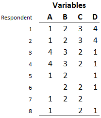
The problem with the MCAR assumption is easy to spot with a simple example. Look at the data to the right, which shows data for 8 people measured on 4 variables. How many clusters can you see? You can probably see 3. The first two rows represent the first cluster. Rows 3 and 4 represent the second cluster. Rows 5 through 8, which represent 50% of the respondents, make up the third cluster. However, if you only use the complete cases - that is, rows 1 through 4 - you can only ever find the first 2 clusters. The third cluster is entirely missing from the data used in complete case analysis.

Dealing with missing data in cluster analysis is almost a nightmare in SPSS. Returning to our case study, where we have no complete cases, if we run it using the default options in SPSS's K-means cluster we get the following error: Not enough cases to perform the cluster analysis. R's kmeans gives essentially the same message, but worded in a way that seems designed to inflict pain on the user: NA/NaN/Inf in foreign function call (arg1).

Complete case analysis followed by nearest-neighbor assignment for partial data

A common way of addressing missing values in cluster analysis is to perform the analysis based on the complete cases, and then assign observations to the closest cluster based on the available data. For example, this is done in SPSS when running K-means cluster with Options > Missing Values > Exclude case pairwise.

This is something of a fig leaf, which is to say that it solves nothing, but the problem gets hidden. Looking at the simple example above, the outcome identifying only two clusters remains. But, respondents represented by rows 5 to 8 will get assigned to one of these clusters (SPSS assigns rows 5 and 7 to the first cluster, and 6 and 8 to the second cluster).

When this method is used in our case study data, we get an error, as none of the respondents have complete data, so the cluster analysis cannot be performed.

Partial data cluster analysis

I have reproduced the simple example data set from above. If you can see the three clusters that I described earlier in my post, you have understood the essence of using partial data when clustering. The idea is as simple as this: group people together based on the data that they have in common. When we do this, we can see that the rows 5 through 8 are identical, except for the unknown missing data.

We can form clusters if we take this approach to our case study. This is a big improvement on the complete case approach. The partial data k-means algorithm that I have used here is one that I have written and made available in an R package on GitHub called flipCluster. By all means you can use it for cluster analysis in R, however, the simplest way to use it is from the menus in Displayr (Insert > More > Segments > K-Means Cluster Analysis). 

If you want to play around with the data in the case study in Displayr, click here.

Replacing missing values with means

A common hack for dealing with missing data is to replace missing values with the mean value of that variable. In the example below, there are two missing values for variable A and 2 for variable C. Each of these variables has an average of 8 (based on those respondents with no missing data for the variable), so we replace the missing values with values of 8.

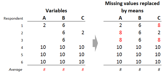
To see the problem with mean imputation, focus on the third row of data. What amount of similarity exists between the respondent and those represented by the other rows? We can only compare based on variable B, as the respondent has no other data. Based on variable B, we would say that this respondents is identical to respondents 1 and 2. The respondent is also clearly different to respondents 4, 5, and 6. Thus, if clustering using partial data, we would end up with respondents 1, 2, and 3, grouped together, and respondents 4 through 6 in another segment.

However, we reach different conclusions when we look at the data where the means replace the missing values. By any sensible criteria, respondent 3 is now more similar to respondents 4, 5, and 6, than to respondents 1 and 2. So, the mean imputation is fundamentally changing the structure of the underlying data. The consequence of this is that when means replace missing values, the final clusters we obtain are, to an some extent, a consequence of the decision to replace the missing values by the means, rather than the data itself.

Imputation

Imputation involves replacing the missing values with sensible estimates of these values. For example, looking at the example above, it may be sensible to replace respondent 2's missing value for variable A with a value of 2. This is sensible because all the information available suggests that respondent 1 and 2 are identical (i.e., they only have one variable in common, B, and both respondents have a 6 for that variable). This is the same logic that underlies using partial data cluster analysis.

It is possible to impute an even better value. The imputation can include variables not used in the cluster analysis. These other variables may be strongly correlated with variable A, allowing us to obtain a superior imputed value. Shrinkage estimators can also be used to reduce the effects of sampling error. For example, while it is true that respondents 1 and 2 are identical based on the only data available, leading to the conclusion that 2 may be a sensible value to impute, it is also true that 3 out of 4 people to have data on variable A have a value of 10.  This implies that 10 may also be a sensible value to impute. Thus, a better estimate may be one that is somewhere between 2 and 10 (or, to be even more precise, between 2 and the average of 8).

The ability to incorporate additional variables combined with using shrinkage estimators means that imputation can outperform partial data cluster analysis. This is because it can take into account relevant information that is ignored by the partial cluster analysis. However, a few things are required in order for this to occur:

• Use a modern imputation algorithm. In practice, this usually means using one of the algorithms available in R, such as those in the mice and mi packages. Most data science and statistics apps have integrations with R (e.g., Displayr, Q, SPSS). Older imputation algorithms will generally perform worse than using partial cluster analysis. This is because the older algorithms can be quite poor (e.g., hot decking), or, make theoretical assumptions that can add considerable noise to the clustering process (e.g. latent class algorithms and algorithms that assume a normal prior).
• The imputation needs to have been done skillfully. It is easy to make mistakes when imputing data.

Consequently, if using imputation, it is usually a good idea to also use partial data cluster analysis and compare and contrast the results (e.g., checking how well they correlate with other data).

Multiple imputation

The best-practice approach for imputation is called multiple imputation. Because you cannot be sure which value is the best to use when imputing, in multiple imputation, you instead work out a range of possible values. You then create multiple data files with different imputed values in each. Some statistical methods can be adjusted to analyze these multiple data files (e.g., regression). However, it does not make sense to use this approach with cluster analysis, as the result would be multiple different cluster analysis solutions, and no rigorous way to combine them.

Summary

Of the five methods considered, three can be outright rejected as being inferior: complete case analysis, complete case analysis followed by nearest-neighbor assignment for partial data, and replacing missing values with means. This is not to say that these methods are always invalid. Ultimately, a cluster analysis solution needs to be judged based on its fitness for a particular problem.

It is therefore possible that these inferior methods can achieve an appropriate solution given the nature of the problem. Having said that, the nature of the inferior methods ultimately cause misrepresentation of the data. This means that, in general, using either partial data cluster analysis or imputation is advisable. If I had little time, I would always choose partial data cluster analysis over imputation. It is both simpler and safer. With sufficient time, I would generally investigate both.

The case study in this Displayr document illustrates the five methods for dealing with missing data in cluster analysis.

Acknowledgements

The data in this case study was provided by GreenBook (GRIT2012/2013).