Please read How to Use Hierarchical Bayes for Choice Modeling in Displayr prior to reading this post.
There are a number of diagnostic tools that you can use to check the convergence of the model. These include looking at the statistics of the parameter estimates themselves, checking trace plots which describe the evolution of the estimates throughout the iterations of the algorithm, and the posterior intervals which show the range of the sampled parameters.
Download our free MaxDiff ebook
Technical overview
Hierarchical Bayes Choice Models represent individual respondent utilities as parameters (usually denoted beta) with a multivariate normal (prior) distribution. The mean and covariance matrix of this distribution are themselves parameters to be estimated (this is the source of the term hierarchical in the name). Hierarchical Bayes uses a technique called Markov Chain Monte Carlo (MCMC) to estimate the parameters, which involves running a number of iterations where estimates of the parameters are generated at each iteration. This iterative sampling of parameters forms what is known as a Markov Chain. In this post I shall use the term sample to refer to a set of estimates of the parameters from a single iteration.
Different software packages have different approaches. The R package, Stan, (used by Q and Displayr) uses a modern form of MCMC called Hamiltonian Monte Carlo. Sawtooth, on the other hand, uses the more old-school Gibbs sampling. My experience is that both approaches get the same answer, but the newer Hamiltonian Monte Carlo is faster for really big problems with lots of parameters. If you wish to use Gibbs Sampling in R, you can do so using the bayesm package. However, in my experience, the resulting models have a worse fit than those from Stan and from Sawtooth.
The samples are generated from those in the previous iteration using a set of rules. The rules are such that once sufficient iterations have been run and the initial samples are discarded, the distribution of the samples matches the posterior distribution of the parameters given prior distributions and observations. In the case of choice-based conjoint, the observations are the respondent’s choices to the alternatives presented to them. By default, Stan discards the first half of the samples. This is known as the warm-up. The latter half of the samples are used to estimate the means and standard errors of the parameters.
The difficult part is knowing how many iterations is sufficient to reach convergence, which I discuss in the next section.
Multiple chains
To take advantage of multi-core processors, multiple Markov chains are run on separate cores in parallel. This has the effect of multiplying the sample size, in return for a slightly longer computation time compared to running a single chain. The more samples, the less sampling error in the results. Here, I am referring to sampling error that results from the algorithm, which is in addition to sampling error from selection of the respondents. In addition, multiple chains result in samples that are less auto-correlated and less likely to be concentrated around a local optima. Having said that, hierarchical Bayes is, in general, less susceptible to local optima than traditional optimization methods due to the use of Monte Carlo methods.
To make full use of computational resources, I recommend that the number of chains is chosen to be equal to or a multiple of the number of logical cores of the machine on which the analysis is run. In Q and Displayr the default of 8 chains is ideal. If you are running your model by R code, you can use detectCores() from the parallel R package. It is important to run multiple chains for the diagnostics discussed in the next section.
Achieving convergence
Formally, a chain is considered to have converged when the sampler reaches stationarity, which is when all samples (excluding the initial samples) have the same distribution. In practice, heuristics and diagnostics plots are used to ascertain the number of iterations required for convergence. The heuristics are based upon two statistics, n_eff and Rhat, which are shown in the parameter statistics output below:
This table includes statistics for the class sizes, estimated means and standard deviations. The off-diagonal covariance parameters are not shown due to the lack of space, and because they are not as important. n_eff is an estimate of the effective sample size (samples of the parameters, not cases). The smaller n_eff, the greater the uncertainty associated with the corresponding parameter. Thus, in the table above, we can see that all the sigma parameters (the standard deviations) tend to have more uncertainty associated with them than the means (this is typical).
The column se_mean shows the standard error of the parameter means, which is computed as sd/sqrt(n_eff), where sd is the standard deviation of the parameter.
Rhat refers to the potential scale reduction statistic, also known as the Gelman-Rubin statistic. This statistic is (roughly) the ratio of the variance of a parameter when the data is pooled across all of the chains to the within-chain variance. Thus, it measures the extent to which chains are reaching different conclusions. The further the value of the statistic from 1, the worse.
As a strategy to achieve convergence, I suggest starting with 100 iterations and set the number of chains equal to the number of logical cores available. The four conditions to check for convergence are:
- No warning messages should appear. Most warning messages are due to insufficient iterations. However if a warning appears indicating that the maximum tree depth has been exceeded, you should increase the maximum tree depth setting from the default of 10 until the warning goes away.
- The estimate of the effective sample size, n_eff, is at least 50 for all values and ideally 100 or more for parameters of interest. A value of 100 is equivalent to specifying that the standard error of the mean is at least an order of magnitude (10 times) less than the standard deviation.
- The potential scale reduction statistic, Rhat, should be less than 1.05 and greater than 0.9 for the parameters of interest.
- Diagnostics plots should not have any unusual features (discussed below).
If any of these conditions are not met, you should re-run the analysis with double the number of iterations, until all conditions have been met. Increasing the iterations beyond this point will increase the precision of the estimates but not drastically change the results. I find that the standard deviation parameters take more iterations to reach convergence than mean parameters. Also, the effective sample size condition tends to be a stricter condition than the one on the potential scale reduction statistic Rhat, so it will be the last to be satisfied.
Refer to the Stan website, and in particular the Stan Modeling Language: User’s Guide and Reference Manual for more information.
Trace plots
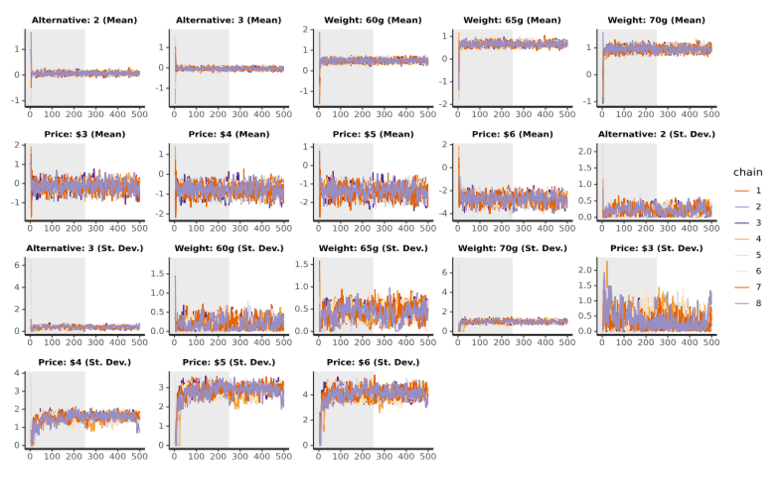
Trace plots show the parameter samples for each chain. The plots below are for means and standard deviations from an example with 500 iterations and 2 chains. The grey halves indicate the warm-up iterations, whereas the second halves of each plot contain the samples that are used to compute the final result. The following are features to look out for that would indicate an issue with the sampling:
- A high degree of correlation between parameters. This would manifest as two or more traces moving in sync.
- A parameter has not stabilized by the end of the warm-up iterations.
- For a particular parameter, there is a chain which is consistently higher or lower than the others.
A practical challenge with these plots on modern machines with more than 2 chains is that often it can be hard to see patterns because all the lines overlap so much.
The above example shows traces which look to converge fairly well. Consider the traces which come from reducing the number of iterations drastically to 50:
Here we see that 50 iterations is not sufficient. Many of the lines have not stabilized after the warm-up stage.
Posterior Intervals
Posterior interval plots show the range of the sampled parameters. The black dot corresponds to the median, while the red line represents the 80% interval, and the thin black line is the 95% interval. There is nothing out of the ordinary in this plot, but I would be concerned if intervals were wide or if the medians were consistently off-center.
Summary
I have provided a brief summary of how hierarchical Bayes for choice modeling works, explained some key diagnostic outputs, and outlined a strategy to ensure convergence. The challenge with hierarchical Bayes is that unlike methods such as latent class analysis, the user needs to verify that the number of iterations is sufficient before proceeding to make any inferences from the results. The convergence criteria listed in this blog post provides a way to ensure the iterations are sufficient, and give us confidence in the answers we obtain. To see the R code used to run hierarchical Bayes and generate the outputs in this blog post, see this Displayr document.