

Root-likelihood (RLH) is a way to measure how well a choice model fits a data set. The RLH is a value ranging between 0 and 1, where a higher value indicates a better fit. It is less susceptible to noise than prediction accuracy but is less commonly used, perhaps because it is harder to conceptualize and interpret. In this article, I will be comparing the performance of Hierarchical Bayes (HB) algorithms from Displayr and Sawtooth. I’ll compare their RLH over four data sets, using both in-sample and holdout data.
How RLH is computed
In order to explain how RLH works, we need to start with the concept of a likelihood. In simple terms, the likelihood is a measurement of how plausible a model’s parameters are, given the available data. In the context of choice modeling, the overall likelihood is the combined likelihoods of the respondent’s questions, where each question’s likelihood is the logit probability for the respondent’s choice.
For example, if there are three alternatives with utilities of 3.4, -0.9, and 1.2, then the logit probabilities are:
![\[ \begin{matrix} &\textrm{Utility}&\textrm{exp(Utility)}&\textrm{Probability}\\ \hline \textrm{Alternative 1} & 3.4 & 30.0 & 30.0/33.7=88.9\%\\ \textrm{Alternative 2} & -0.9 & 0.41 & 0.41/33.7=1.2\%\\ \textrm{Alternative 3} & 1.2 & 3.32 & 3.32/33.7=9.9\%\\ \hline \textrm{Sum}&&33.7&100\% \end{matrix} \]](https://www.displayr.com/wp-content/ql-cache/quicklatex.com-3e2bc1ce8ee8c0638845be437db0d415_l3.png "Rendered by QuickLaTeX.com")
So if the respondent chose Alternative 1, the likelihood for this question is 88.9%. The likelihood for the entire model is simply the product of the likelihoods for every question. The RLH is computed by taking the nth root of the likelihood, where n is the number of respondent questions. This is equivalent to the geometric mean of the likelihoods of the respondent questions (i.e. RLH is a kind of “average” likelihood of each question). An RLH can also be computed for a respondent as the geometric mean of the likelihoods of just their questions.
A null model where utilities are the same for all alternatives (i.e. a model that randomly chooses alternatives with equal probability) has an RLH of 1/k, where k is the number of alternatives. A model with a good fit to the data should have a larger RLH than this. However, when the fit is worse, such as when predicting holdout data, it is not unusual to have an RLH below 1/k. This is because of the nature of the geometric mean: small values have a large impact on the mean, dragging it lower than would be the case with the arithmetic mean.
For example, suppose there are three questions and the probabilities of the chosen alternatives are 0.99, 0.005, and 0.005. If the model correctly predicts the first two choices, then the predictive accuracy is 67%. However, the RLH is much lower at 0.17 — (0.99 * 0.99 * 0.005)^(1/3) = 0.17 — which is less than the null model RLH of 0.33. The null model has a higher RLH even though it only has a 33% accuracy.
Methodology
I ran Hierarchical Bayes (HB) using Displayr and Sawtooth on four choice model data sets, which contained data on cruise ship holiday, eggs, chocolate, and fast food preferences. The cruise ship data set was used in a modeling competition in 2016 run by Sawtooth Software, and the other data sets were collected by Displayr.
One question was left out per respondent to be used as the holdout, and the analysis was run with the default settings in both Displayr and Sawtooth. The RLH was computed from respondent parameters estimated by the model, and charts of the results were created with Displayr.
In-sample results
The grid of scatterplots below compares the in-sample RLH for the Displayr and Sawtooth HB models. Each data point represents the RLH for a single respondent, and the results are compared for all four data sets.
In all four charts, the RLH is concentrated around the top right quadrant. This indicates a good in-sample fit to the data. The Displayr and Sawtooth RLH are somewhat correlated, but the Sawtooth RLH are larger on average.
The next chart shows the overall in-sample RLH for the same data sets. The in-sample RLH from Sawtooth is larger than those from Displayr for all four data sets, which suggests that the Sawtooth HB model has a better in-sample fit than the Displayr model.
However, this could be a sign of overfitting to the data. We can test this by using the holdout data.
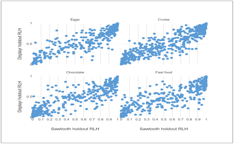
The final chart shows that the Displayr holdout RLH is higher than those of Sawtooth for all four data sets. This confirms that the Sawtooth models are overfitting more than the Displayr models.
The RLH for both models is lowest for the chocolate and fast food data sets since they have a high number of attributes relative to the number of questions, making them more prone to overfitting. There are four alternatives per question, which means that the null model Chocolate data set has an RLH of 0.25. The Sawtooth model has an RLH of just 0.19.
Also, note that the difference in RLH between the Displayr and Sawtooth models is largest for chocolate and fast food. This is the case for both for in-sample and holdout. From this, we can conclude that Sawtooth overfits more on data sets that are already prone to overfitting.
Conclusion
In this article, I described how RLH is computed and compared the performance of Displayr and Sawtooth HB using this metric. I found that Sawtooth HB overfitted to all four data sets more than Displayr, especially on data sets prone to overfitting. To mitigate the issue of overfitting, the default priors can be changed to “shrink” the model. But it requires a solid understanding of the underlying HB model, as well as a lot of trial and error, to correctly set the priors. Therefore it is important that default priors for HB choice modeling software are appropriately set to minimize this issue.