
When creating a predictive model, there are two types of predictors (features): numeric variables, such as height and weight, and categorical variables, such as occupation and country. In this post I go through the main ways of transforming categorical variables when creating a predictive model (i.e., feature engineering categorical variables). For more information, also check out Feature Engineering for Numeric Variables.
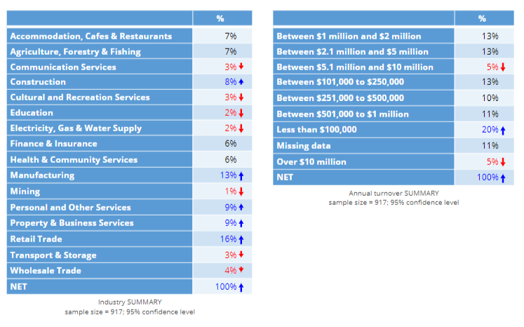
In this post I work my way through a simple example, where the outcome variable is the amount of gross profit that a telco makes from each of a sample of 917 of its customers, and there are two predictors: industry and the turnover of the company. The goal of the predictive model is to identify which industries and company sizes to focus its efforts on. Tables showing the proportion of customers in each of the categories for the two features (aka predictor variables) are shown below.
Using the predictive model’s in-built tools for categorical variables
The simplest approach to analyzing such data is to just select the predictor variables in whatever software you are using and let the software decide to automatically treat the data how it wants. If you are using well-written software this will often be an OK option, and will likely use one-hot encoding in the background.
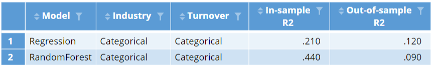
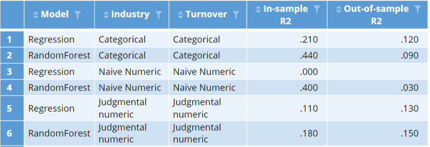
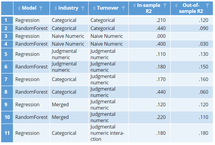
The table below shows the r-squared statistics for both a linear regression and a random forest. The random forest does a much better job at predicting profit with the data used to fit the models (this is shown in the In-sample R2 column). This is not surprising, as this model is much more flexible, so can typically fit a specific data set better than a standard linear regression. However, in data not used to fit the model, this result reverses, with the regression performing better. In both cases the out-of-sample accuracy is much, much, worse. (See How to do Logistic Regression in Displayr for a discussion regarding the need for saving data for use in checking a model). This is a general issue with categorical predictors: the more categories, the more likely the models will over-fit (produce much better in-sample than out-of-sample fits).
Treating the predictors as numeric variables
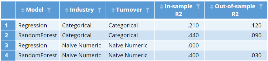
An alternative to treating the data as categorical is to treat it as numeric. This entails assigning a value of 1 to the first category, 2 to the second category, and so on (e.g., 1 to Accommodation, Cafes & Restaurants, a 2 to Agriculture, Forestry & Fishing, etc.). The bottom two lines of the table below show the results of the models when the variables are treated as numeric. After this feature engineering, the linear regression essentially fails, with an r-squared of 0 in the data used to estimate the model and an error when computing the out-of-sample fit (the model produced worse-than-random predictions). The random forest does better, but the out-of-sample fit is substantially worse. We can learn from this that it is important to avoid unintentionally treating categorical predictors as numeric variables when creating predictive models (this may sound obvious, but it can be easy to do this inadvertently if you do not know to avoid the problem).
Judgmental encodings
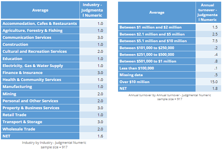
There is an obvious ordering to the turnover categories below. An alternative way of analyzing the turnover data is to treat it as numeric, but use judgment to assign values to the data. For example, we could use consecutive integers, assigning a 1 to the lowest category, a 2 to the next lowest, and so on. Alternatively, we could assign midpoints or some other value. In the two tables below I have assigned values to each of the two predictor variables. In the case of the turnover data, the judgments seem reasonably sound to me (other than for Missing data), but for the industry data the encoding has little more than guesswork to justify it.
When coming up with your own encodings, there are a few rules:
- The results of predictive models are not super-sensitive to the choices. For example, we could assign a value of 0, .05, or 1 to the Less than $100,000 category and it will make no difference, and even with the Over $10 million category, any of 10, 15, or 20 will likely not make a huge impact.
- You should not look at relationship between the predictor variable and the outcome variable when forming the encoding. If you do, you will overfit your model (create a model that looks good initially but predicts poorly).
The results of the models with the judgmental encoding are shown below. Each of these models are relatively poor in-sample. This is to be expected, as the models with numeric predictor variables are less flexible. However, the out-of-sample performance of these two models is the best we have seen. It is pretty common to find this type of result: incorporating judgment into modeling tends to lead to better models.
Mixed judgment and categorical
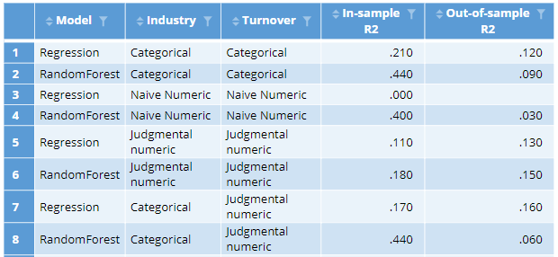
The judgments regarding the encoding of turnover are relatively easy to defend. The ones made about industry are not. This suggests we should consider treating industry as a categorical variable, but use turnover with its judgmental encoding. The resulting two models are shown at the bottom of the table below. Looking at the in-sample r-squareds, we can see that the random forest has improved markedly on the training data, as now it can explore all possible combinations of industry and how they interact with turnover. However, its out-of-sample performance has become abysmal. By contrast, the best of the models is now our regression model, with the categorical industry and judgmentally-encoded turnover. This highlights an important practical issue with feature engineering: its effect varies depending on which predictive algorithm we use.
.
Merging categories
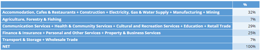
The massive degree of overfitting we are seeing with the random forest is because we have so many categories of industry, which leads to too many possible ways of combining industry together. We can limit the number of possible combinations by using judgment to merge some of the categories. I’ve used my own judgment to merge the categories as shown in the table below. For the same reasons described in the earlier section on judgmental encodings, it is important not to look at the outcome variable when working out which categories should be merged. By contrast, it is appropriate to look at the sizes of the categories, as categories with small samples tend to be unreliable and often benefit from being merged.
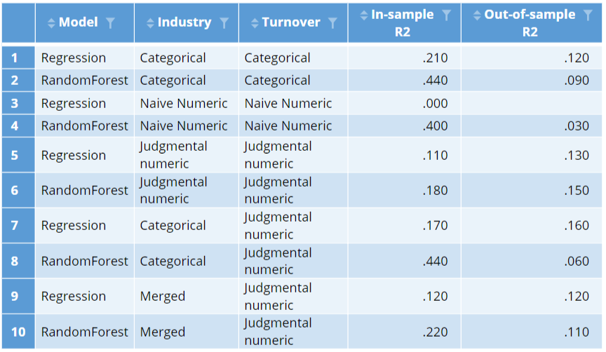
The in-sample r-squared of both the regression and the random forest declines. This is to be expected. By merging the categories we have guaranteed that the in-sample fit will decline. In the case of the random forest, the out-of-sample r-squared is better than the previous model, suggesting that the merging of the categories was not completely hopeless. However, the best model remains the regression model with all the industry categories and the judgmentally-encoded turnover variable.
Interactions
An interaction is a new variable, or set of variables, created by multiplying together predictor variables. To explain how they work with categorical variables it is necessary to delve a little into the detail of how predictive models deal with categorical variables.
The industry variable has 16 categories and the turnover variable has nine. When most (but not all) machine learning and statistical methods analyze a categorical variable they perform one-hot coding in the background. In the case of our 16 categories for industry, what this means is that 15 numeric variables are created and included in the model, one for all but the first of the categories. These are given a value of 1 when the data contains that category and a value of 0 otherwise. (Such variables are also known as dummy variables.) So, when we are estimating our model with industry and turnover, we are estimating 15 and 8 variables in the background to represent these two categorical variables.
A standard interaction of industry by age would create 16 * 8 = 128 variables in the background (it’s actually a bit more complicated than this, but hopefully you get the idea). This considerably improves the in-sample fit, but tends to raise lots of problems in the out-of-sample predictive accuracy, as often combinations of categories that exist in the data used to estimate the model do not exist in the data set used to validate the model, and vice versa. The solution, then, when you have categorical variables with large numbers of categories and wish to create interactions, is to use merged variables when creating interactions and/or numerically encoded variables.
While you can create the interactions by hand, most predictive modeling software has automatic tools to make this easy. In Displayr, we do this by editing the R code (Object Inspector > Properties > R CODE), and adding a * or a : to the formula, as can be seen in the screenshot below (see Feature Engineering for Numeric Variables for the distinction between : and *).

The resulting model, shown at the bottom of the table has the best out-of-sample r-squared of all of the models considered so far. The out-of-sample r-squared is as good as the in-sample r-squared, but this is just good luck and is not the norm.
This post has provided a tour of some of the options for engineering categorical variables (features) when creating predictive models. The interesting thing to note is the substantial impact that can be achieved by judiciously transforming categorical variables, with the resulting model substantially better than the default models that can be obtained without transforming the data.
Explore the original dashboard
If you want to look at the various analyses discussed in this post in more detail (e.g., looking at the coefficients of all the models), click here to view the Displayr document that contains all the work. If you want to reproduce these analyses yourself, either with this data or some other data, please check out:
- How to do Logistic Regression in Displayr
- Feature Engineering in Displayr
- Feature Engineering for Numeric Variables
Click the button above to edit and explore the original analyses!