
How To Add Trend Lines in R | Step-By-Step Guide
When you are conducting an exploratory analysis of time-series data, you'll need to identify trends while ignoring random fluctuations in your data. There are multiple ways to solve this common statistical problem in R by estimating trend lines. We'll show you how in this article, as well as how to visualize it using the Plotly package.
1. Global trend lines
One of the simplest methods to identify trends is to fit a ordinary least squares regression model to the data. The model most people are familiar with is the linear model, but you can add other polynomial terms for extra flexibility. In practice, avoid polynomials of degrees larger than three because they are less stable.
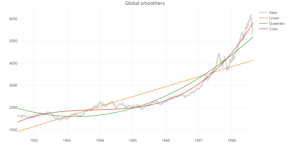
Below, we use the EuStockMarkets data set (available in R data sets) to construct linear, quadratic and cubic trend lines.
data("EuStockMarkets")
xx = EuStockMarkets[,1]
x.info = attr(xx, "tsp")
tt = seq(from=x.info[1], to = x.info[2], by=1/x.info[3])
data.fmt = list(color=rgb(0.8,0.8,0.8,0.8), width=4)
line.fmt = list(dash="solid", width = 1.5, color=NULL)

ti = 1:length(xx)
m1 = lm(xx~ti)
m2 = lm(xx~ti+I(ti^2))
m3 = lm(xx~ti+I(ti^2)+I(ti^3))

require(plotly)
p.glob = plot_ly(x=tt, y=xx, type="scatter", mode="lines", line=data.fmt, name="Data")
p.glob = add_lines(p.glob, x=tt, y=predict(m1), line=line.fmt, name="Linear")
p.glob = add_lines(p.glob, x=tt, y=predict(m2), line=line.fmt, name="Quadratic")
p.glob = add_lines(p.glob, x=tt, y=predict(m3), line=line.fmt, name="Cubic")
p.glob = layout(p.glob, title = "Global smoothers")
print(p.glob)
2. Local smoothers
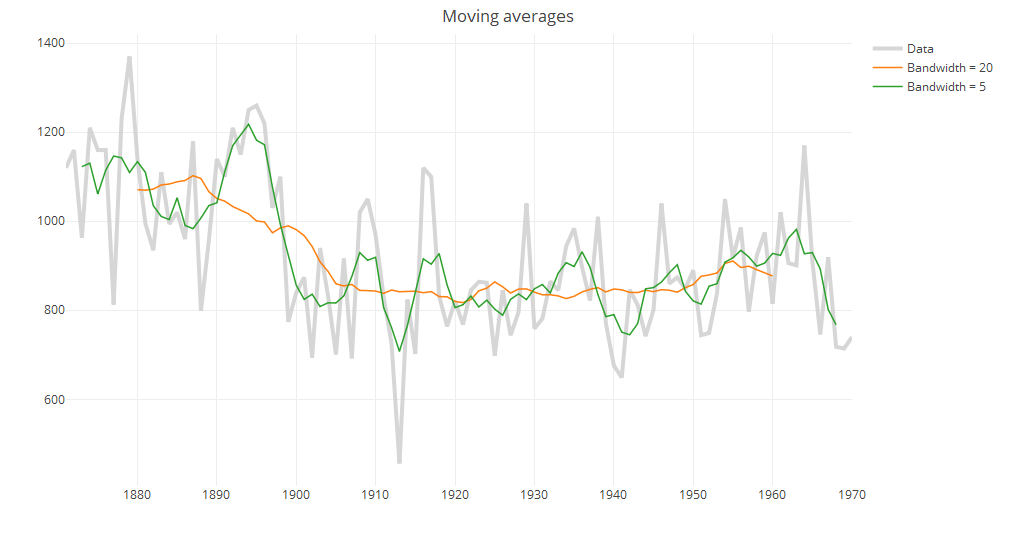
Global models assume that the time series follows a single trend. For many data sets, however, we would want to relax this assumption. In the following section, we demonstrate the use of local smoothers using the Nile data set. It contains measurements of the annual river flow of the Nile over 100 years and is less regular than the EuStockMarkets data set.
i. Moving averages
The moving average (also known as running mean) method consists of taking the mean of a fixed number of nearby points. Even with this simple method we see that the question of how to choose the neighborhood is crucial for local smoothers. Increasing the bandwidth from 5 to 20 suggests that there is a gradual decrease in annual river flow from 1890 to 1905 instead of a sharp decrease at around 1900.
Many packages include functions to compute the running mean such as caTools::runmean and forecast::ma, which may have additional features, but filter in the base stats package can be used to compute moving averages without installing additional packages.
data("Nile")
xx = Nile
x.info = attr(xx, "tsp")
tt = seq(from=x.info[1], to = x.info[2], by=1/x.info[3])

rmean20 = stats::filter(xx, rep(1/20, 20), side=2)
rmean5 = stats::filter(xx, rep(1/5, 5), side=2)

require(plotly)
p.rm = plot_ly(x=tt, y=xx, type="scatter", mode="lines", line=data.fmt, name="Data")
p.rm = add_lines(p.rm, x=tt, y=rmean20, line=line.fmt, name="Bandwidth = 20")
p.rm = add_lines(p.rm, x=tt, y=rmean5, line=line.fmt, name="Bandwidth = 5")
p.rm = layout(p.rm, title = "Running mean")
print(p.rm)
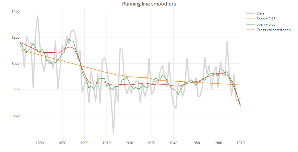
ii. Running line smoothers
The running line smoother reduces the bias by fitting a linear regression in a local neighborhood of the target value. A popular algorithm using the running line smoother is Friedman’s super smoother supsmu, which by default uses cross-validation to find the best span.
rlcv = supsmu(tt, xx)
rlst = supsmu(tt, xx, span = 0.05)
rllt = supsmu(tt, xx, span = 0.75)

p.rl = plot_ly(x=tt, y=xx, type="scatter", mode="lines", line = data.fmt, name="Data")
p.rl = add_lines(p.rl, x=tt, y=rllt$y, line=line.fmt, name="Span = 0.75")
p.rl = add_lines(p.rl, x=tt, y=rlst$y, line=line.fmt, name="Span = 0.05")
p.rl = add_lines(p.rl, x=tt, y=rlcv$y, line=line.fmt, name="Cross-validated span")
p.rl = layout(p.rl, title = "Running line smoothers")
print(p.rl)
iii. Kernel smoothers
An alternative approach to specifying a neighborhood is to decrease weights further away from the target value. These estimates are much smoother than the results from either the running mean or running line smoothers.
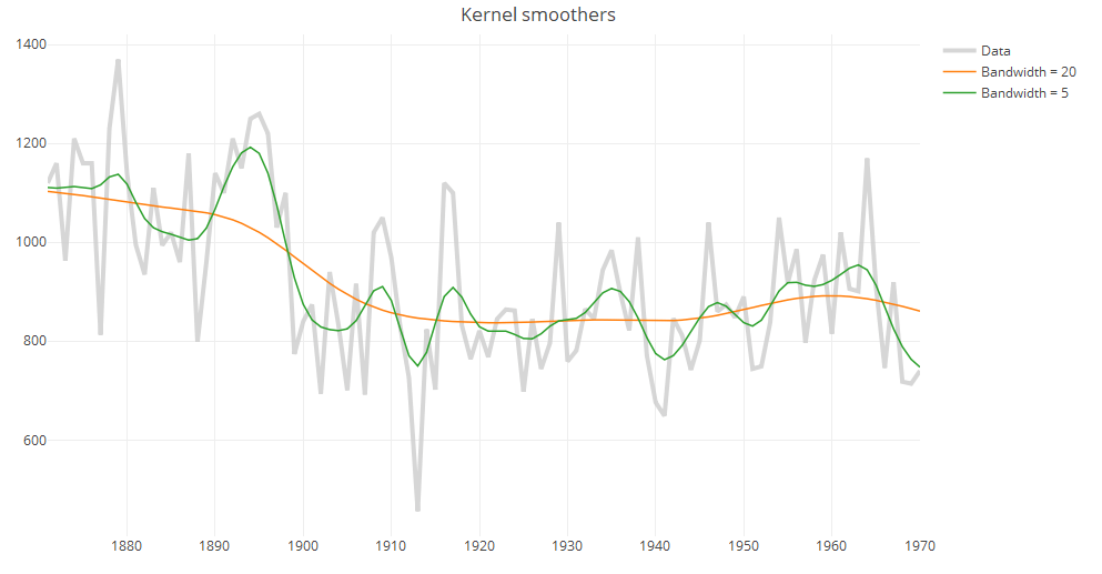
ks1 = ksmooth(tt, xx, "normal", 20, x.points=tt)
ks2 = ksmooth(tt, xx, "normal", 5, x.points=tt)

p.ks = plot_ly(x=tt, y=xx, type="scatter", mode="lines", line=data.fmt, name="Data")
p.ks = add_lines(p.ks, x=ks1$x, y=ks1$y, line=line.fmt, name="Bandwidth = 20")
p.ks = add_lines(p.ks, x=ks1$x, y=ks2$y, line=line.fmt, name="Bandwidth = 5")
p.ks = layout(p.ks, title = "Kernel smoother")\
print(p.ks)
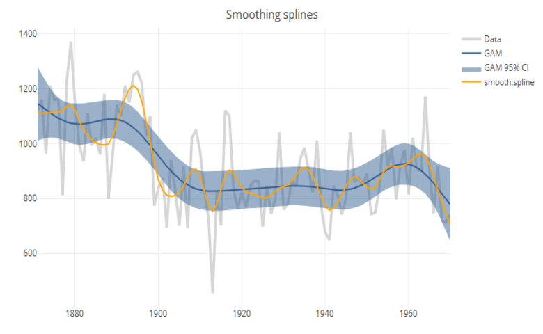
iv. Smoothing splines
Splines consist of a piece-wise polynomial with pieces defined by a sequence of knots where the pieces join smoothly. A smoothing splines is estimated by minimizing a criterion containing a penalty for both goodness of fit, and smoothness. The trade-off between the two is controlled by the smoothing parameter lambda, which is typically chosen by cross-validation.
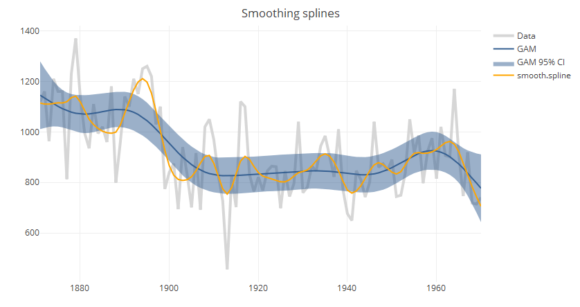
In the base package, smooth.spline can be used to compute splines, but it is more common to use the GAM function in mgcv. Both functions use cross-validation to choose the default smoothing parameter; but as seen in the chart above, the results vary between implementations. Another advantage to using GAM is that it allows estimation of confidence intervals.
require(mgcv)
sp.base = smooth.spline(tt, xx)
sp.cr = gam(xx~s(tt, bs="cr"))
sp.gam = gam(xx~s(tt))
sp.pred = predict(sp.gam, type="response", se.fit=TRUE)
sp.df = data.frame(x=sp.gam$model[,2], y=sp.pred$fit,
                    lb=as.numeric(sp.pred$fit - (1.96 * sp.pred$se.fit)),
                    ub=as.numeric(sp.pred$fit + (1.96 * sp.pred$se.fit)))
sp.df = sp.df[order(sp.df$x),]

pp = plot_ly(x=tt, y=xx, type="scatter", mode="lines", line=data.fmt, name="Data")
pp = add_lines(pp, x=tt, y=sp.pred$fit, name="GAM", line=list(color="#366092", width=2))
pp = add_ribbons(pp, x=sp.df$x, ymin=sp.df$lb, ymax=sp.df$ub, name="GAM 95% CI", line=list(color="#366092", opacity=0.4, width=0))
pp = add_lines(pp, x=tt, y=predict(sp.base)$y, name="smooth.spline", line=list(color="orange", width=2))
pp = layout(pp, title="Smoothing splines")
print(pp)
v. LOESS
LOESS (Locally Estimated Scatterplot Smoother) combines local regression with kernels by using locally weighted polynomial regression (by default, quadratic regression with tri-cubic weights). It also allows estimation of approximate confidence intervals. However, it is important to note that unlike supsmu, smooth.spline or gam, loess does not use cross-validation. By default, the span is set to 0.75; that is, the estimated smooth at each target value consists of a local regression constructed using 75% of the data points closest to the target value. This span is fairly large and results in estimated values that are smoother than those from other methods.
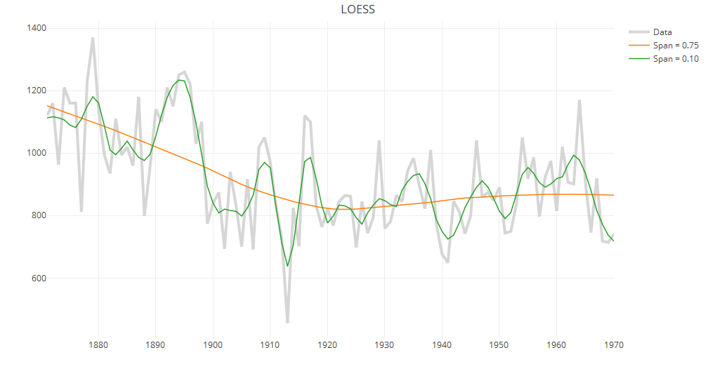
ll.rough = loess(xx~tt, span=0.1)
ll.smooth = loess(xx~tt, span=0.75)

p.ll = plot_ly(x=tt, y=xx, type="scatter", mode="lines", line=data.fmt, name="Data")
p.ll = add_lines(p.ll, x=tt, y=predict(ll.smooth), line=line.fmt, name="Span = 0.75")
p.ll = add_lines(p.ll, x=tt, y=predict(ll.rough), line=line.fmt, name="Span = 0.10")
p.ll = layout(p.ll, title="LOESS")
print(p.ll)
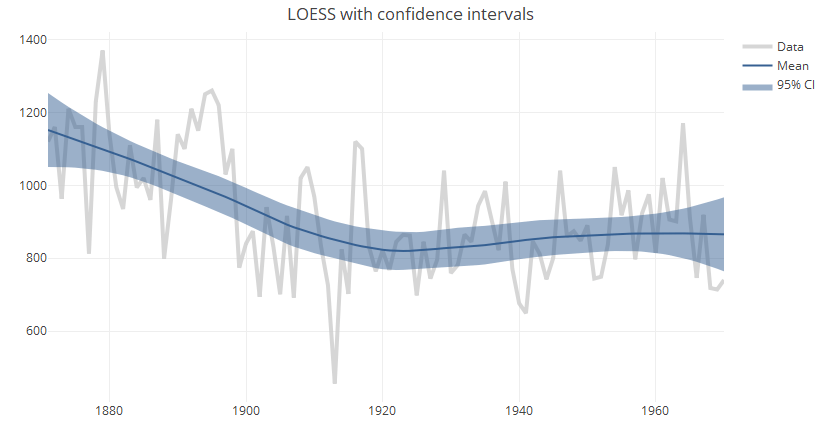
ll.smooth = loess(xx~tt, span=0.75)
ll.pred = predict(ll.smooth, se = TRUE)
ll.df = data.frame(x=ll.smooth$x, fit=ll.pred$fit,
lb = ll.pred$fit - (1.96 * ll.pred$se),
ub = ll.pred$fit + (1.96 * ll.pred$se))
ll.df = ll.df[order(ll.df$tt),]

p.llci = plot_ly(x=tt, y=xx, type="scatter", mode="lines", line=data.fmt, name="Data")
p.llci = add_lines(p.llci, x=tt, y=ll.pred$fit, name="Mean", line=list(color="#366092", width=2))
p.llci = add_ribbons(p.llci, x=ll.df$tt, ymin=ll.df$lb, ymax=ll.df$ub, name="95% CI", line=list(opacity=0.4, width=0, color="#366092"))
p.llci = layout(p.llci, title = "LOESS with confidence intervals")
print(p.llci)
Sign up for Displayr