Shapley regression and Relative Weights are two methods for estimating the importance of predictor variables in linear regression. Studies have shown that the two, despite being constructed in very different ways, provide surprisingly similar scores((Grömping, U. (2015). Variable importance in regression models, WIREs Comput Stat 7, 137-152.))((Lebreton, J.M., Ployhart, R.E., & Ladd, R.T. (2004). A Monte Carlo Comparison of Relative Importance Methodologies. Organizational Research Methods 7, 258 – 282.)). As the computational expense of Shapley regression by far outweighs that of Relative weights, and if the two yield essentially the same results, then you can consider Relative Weights a strong alternative to Shapley. In this blog post, I explore the relationship between the two methods.
Shapley regression
Shapley regression (also known as dominance analysis or LMG) is a computationally intensive method popular amongst researchers. To describe the calculation of the score of a predictor variable, first consider the difference in R2 from adding this variable to a model containing a subset of the other predictor variables. Then, obtain the score by computing these differences over all possible subsets and averaging. Whilst simple in principle, the number of cases to consider doubles with every additional predictor variable. Thus, a model with 20 variables will have over 1 million different cases. This results in a non-trivial calculation, even on a modern desktop computer.
To demonstrate the calculation of a Shapley, consider a three-variable regression of y on X1, X2, and X3. Using real data, the R2 for the regressions run on the predictor subsets are:
[
begin{array}{c|c|c}
textrm{Model}&textrm{Predictors}&R^2\
hline
0&textrm{none}&0\
1&X_1&0.1064\
2&X_2&0.1254\
3&X_3&0.1288\
{1,2}&X_1,X_2&0.1807\
{1,3}&X_1,X_3&0.1700\
{2,3}&X_2,X_3&0.1873\
{1,2,3}&X_1,X_2,X_3&0.2144
end{array}
]
Calculate the Shapley score for X1 by averaging the differences in R2 of models with and without X1 as a predictor variable:
[
frac13(R^2_{1,2,3}-R^2_{2,3})+frac16(R^2_{1,2}-R^2_2)+frac16(R^2_{1,3}-R^2_3)+frac13(R^2_1-R^2_0)=0.0606
]
Note that weights are chosen such that the weight for adding X1 to a model with two predictors equates to the total weight for adding X1 to a model with one predictor. This is also the same as the weight for adding X1 to a model with no predictors. This general pattern holds for models with more predictors. Similarly, the Shapley scores for X2 and X3 are:
[
frac13(R^2_{1,2,3}-R^2_{1,3})+frac16(R^2_{1,2}-R^2_1)+frac16(R^2_{2,3}-R^2_3)+frac13(R^2_2-R^2_0)=0.0788
]
[
frac13(R^2_{1,2,3}-R^2_{1,2})+frac16(R^2_{1,3}-R^2_1)+frac16(R^2_{2,3}-R^2_2)+frac13(R^2_3-R^2_0)=0.0751
]
Relative Weights
An alternative to Shapely regression, Relative Weights((Johnson, J.W. (2000). A heuristic method for estimating the relative weight of predictor variables in multiple regression. Multivariate behavioral research 35, 1-19.)) produces similar scores with much faster computation. This method transforms the predictor variables to a set of orthogonal variables (not correlated with each other). When the outcome variable is regressed on these orthogonal variables, the squared coefficients from the regression represent each orthogonal variable’s contribution to the R2. The matrix from the initial transformation is then used to convert these contributions to importance scores of the original predictor variables. This procedure involves running a fixed number of linear algebra operations whose complexity only increases as a square of the number of variables, rather than exponentially, making it much faster to run.
Analytical expressions of scores
I sought to find analytical expressions for the two methods to see how they differ. Since they are identical for models with two predictors, I consider models with three predictors: models with more predictors makes analysis much more complicated. Comparing models with three predictors will provide us with insight into how the methods differ in general.
Neither method depends on the offset and scale of the outcome and predictor variables. Therefore, it can be assumed that they are normalized to have a mean of zero and a variance of one. As a result, two methods can be calculated from the correlations between the predictor variables and the regression coefficients.
I managed to derive a general analytical expression for Shapley scores for models with three predictors, but unfortunately it is too long to display in its entirety in this blog post and there is no easy interpretation of it as far as I can tell. I display the first six terms for the Shapley score of the first predictor below, with another 47 terms not shown here:
[frac16left(frac{4{{beta}_{2}}{{beta}_{3}}{{{{rho}_{23}}}^{3}}}{1-{{{{rho}_{23}}}^{2}}}+frac{4{{beta}_{1}}{{beta}_{3}}{{rho}_{13}}{{{{rho}_{23}}}^{2}}}{1-{{{{rho}_{23}}}^{2}}}+frac{4{{beta}_{1}}{{beta}_{2}}{{rho}_{12}}{{{{rho}_{23}}}^{2}}}{1-{{{{rho}_{23}}}^{2}}}+frac{2{{{{beta}_{3}}}^{2}}{{{{rho}_{23}}}^{2}}}{1-{{{{rho}_{23}}}^{2}}}+frac{2{{{{beta}_{2}}}^{2}}{{{{rho}_{23}}}^{2}}}{1-{{{{rho}_{23}}}^{2}}}+frac{4{{{{beta}_{1}}}^{2}}{{rho}_{12}}{{rho}_{13}}{{rho}_{23}}}{1-{{{{rho}_{23}}}^{2}}}+ldotsright),]
where $beta$ represents the vector of coefficients and $rho$ the correlation matrix of predictors.
Deriving a general expression for Relative Weights turned out to be too difficult even with the assistance of computer algebra system. The problem becomes much more tractable when I fix values for the correlations and coefficients. Therefore I explore how the two methods differ when fixing all but one of the values.
Varying correlation between predictors
In the first comparison I set the values of the coefficients $beta$ and the correlation matrix of the predictors $rho$ to be:
[
beta=
left[ {begin{array}{c}
0.5\
-0.2\
0.05end{array} } right]
quadtextrm{and}quad
rho=
left[ {begin{array}{ccc}
1 & rho_{12} & 0.5 \
rho_{12} & 1 & 0.5 \
0.5 & 0.5 & 1end{array} } right]
]
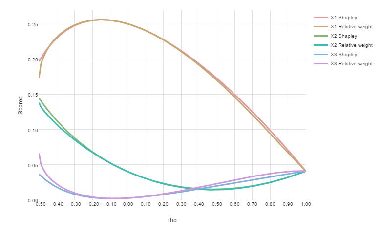
where $rho_{12}$ is allowed to vary. I chose these values to be similar to those found in a typical regression model. Although a correlation coefficient may range from -1 to 1, $rho_{12}$ is further constrained by the requirement that the matrix $rho$ needs to be a valid correlation matrix. This limits the range of $rho_{12}$ to -0.5 to 1. The chart below plots the Shapley scores and Relative Weights over this range, for the three predictor variables X1, X2 and X3:
Note the remarkable similarity of the two methods for most values of $rho_{12}$, except near -0.5. At this point, the correlation matrix becomes more pathological and unlikely to be encountered in the real-world. Beyond 0.5, $rho$ is no longer a valid correlation matrix. If I sort the predictor variables by their scores, the order of the variables is almost identical between methods. The order only differs where variable lines intersect. For example, between values of 0.65 to 0.68 for $rho_{12}$, the scores for the second predictor variable X2 are less than the Relative Weights of the third predictor variable X3 but more than the Shapley scores for X3. In any case, the order of variables within this range is not important as the scores are very close to each other and variables should be considered equivalent for comparison purposes.
Varying a regression coefficient
In the second comparison I set the values of the coefficients $beta$ and the correlation matrix of the predictors $rho$ to
[
beta=
left[ {begin{array}{c}
beta_1\
0.1\
-0.4end{array} } right]
quadtextrm{and}quad
rho=
left[ {begin{array}{ccc}
1 & 0.5 & 0.2 \
0.5 & 1 & -0.3 \
0.2 & -0.3 & 1end{array} } right]
]
where I am now varying the regression coefficient $beta_1$ instead of a correlation coefficient. Again, I chose these values to be similar to those found in a typical regression model. In the chart below, we have restricted the range of $beta_1$ such that the sum of the scores (equal to the R2) is no more than 1:
The two methods are again very similar and the order of variables is the same except over a small range of $beta_1$. The two methods differ most when the magnitude of $beta_1$ is largest, but even then, inferences made using the two methods are unlikely to differ.
In summary, my findings match those of previous studies comparing these methods, which used models with more predictors on specific data sets. Consequently, you can substitute Shapley regression with Relative Weights and vice versa.
Displayr is your complete solution for weighting survey data. Start your free trial today.
Acknowledgements
The outputs shown above use plotly.