

Modern conjoint analysis methods estimate both the utilities of people, and also how much certainty we have about these estimates. Consequently, analyses of the resulting data should be performed in a way that takes into account this uncertainty. Fortunately, with hierarchical Bayesian methods (HB), this is quite simple. In this post I provide a worked example using Displayr, but the basic principle is applicable with any HB model.
Step 1: Save the draws (iterations)
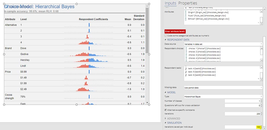
HB models start by making a guess at the utilities, via random number generation typically, and then work to improve on these estimates. Each attempt to improve the estimates of the utilities is known as an iteration or draw (as in “drawing” a ball from an urn, for those of you that have studied probability theory). Once the HB model has converged, any subsequent draws can be used in analysis. Most of the standard outputs from Bayesian analysis are just computed as averages of the draws that occur after convergence. In the output below, the Mean column is just the average of the draws. The histograms are computed in two stages. First, the average draw is computed for each person. The histograms are then of these averages.
By default, some HB software does not actually save the draws after computing the statistics. So, the first step is to tell the software to save these draws. In Displayr, this is done by clicking on the model and setting Inputs > SIMULATION > Iterations saved per individual to, say, 100. Note that when you do this the model will have to re-run, so it is best to do this at the beginning. Also, keep in mind that these draws take up a lot of memory, so if you get weird error messages about memory, you should reduce the number of draws. As few as 10 can be OK.
Step 2: Extract the draws
Once you have saved the draws, you need to extract them for analysis. In Displayr, this can be done using Insert > R Output, and pasting in the following code, where you may need to change the name of your model (mine is called choice.model, which is the name of the first conjoint analysis model created in a Displayr document), and the name of the utility (draws of a parameter) that you wish to extract. The resulting output is two-dimensional, where each column represents the draws for a respondent, and each row represents the draws.
Step 3: Understand the distinction between the draws and the respondent utilities
Each respondent’s utility is just the average of their draws (the columns in the table above). These utilities have a few different names, including respondent coefficients or individual-level parameters. The histograms above show the utilities for each of the attribute levels. As each respondent’s utility is an average, it is necessarily the case that the variation between respondents’ utilities must be less than the variation between the draws. This can be seen in the density plots below. The top one shows the distribution of the respondents utilities, and corresponds to the Price: $2.49 histogram shown in the first plot. The bottom density plot shows the distribution of all the draws.
It is not an accident that the distribution of the draws looks normal. This is an assumption of the HB model. There are ways of varying this assumption, but it is the norm to make this assumption, even in situations where on face value it does not make sense, such as in this case. The reason it doesn’t make sense on face value is that a normal distribution implies that it is possible for people to have a positive utility approaching infinity for the price of $2.49, and this isn’t at all consistent with economic theory. In practice, this tends not to be a problem.
Step 4: Perform calculations using the draws
If you look at the density plot for the draws, we can see that a significant amount of them are above 0. We can compute the exact proportion in Displayr as 19%, by inserting an R Output and using:
In the case of the respondent means, by contrast, we have only 6% that are above 0.
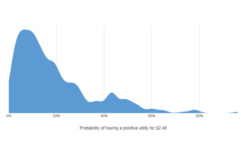
While it would be tempting to exclude these 6% of respondents as having irrational data, to do so ignores the uncertainty we have in the data. How confident would we want to be before deciding to throw out a respondent? The density plot below shows distribution of people in terms of the number of draws that they have which are positive. The vast majority of people have probabilities less than 50%, with the mode being less than 10%, suggesting that for most people we can be confident that they are averse to paying more for chocolate.
These are the calculations required for generating the data plotted in the density plot (Insert > Visualization > Density Plot):
I’d want to give a respondent the benefit of the doubt, and only exclude their data if I was 90% sure that their data showed they have a positive utility for price. If we do this calculation, we discover that there is only 0.3% of respondents (1 person), that we need to throw out based on their having provided irrational pricing data.
One of the many cool things about Bayesian statistics is it is relatively simple. Once you have the draws, you make conclusions that take into account uncertainty, with simple calculations like these.
You can view these calculations, hooked up to the raw data and models in Displayr, by clicking here.
