
It shows how likely people are to make purchases at different price points. There are lots of different ways of estimating demand curves. In this post, I explain the basics of doing so from a conjoint study using Displayr.
Example demand curve
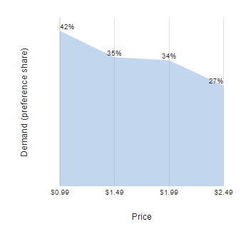
Below is a demand curve from a choice-based conjoint study of the chocolate market. It shows preference share for a 2-ounce Hershey milk chocolate bar.
Preparation: Creating the model and simulator
Before computing the demand curve you need a simulator. The most straightforward way of doing this is to create a model using Insert > More > Conjoint/Choice Modeling > Hierarchical Bayes, followed by Insert > More > Conjoint/Choice Modeling > Simulator.
Manually creating the demand curve
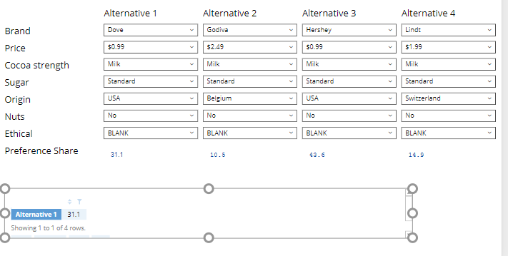
The simplest way to create a demand curve is to manually run each scenario of interest in your simulator. Let’s say we wanted to create the demand curve for Hershey. We would set each of the alternatives to the desired attribute levels, with Hershey at the lowest price point, and make a note of Hershey’s market share. Then, we would increase Hershey’s price to the next price point and make a note of that share, and so on. You can then use Home > Enter Table to create a table of these data points (with price in the first column and market share in the second) and hook it up to a visualization.
Code based-creation of a demand curve
There are several situations where manually creating the demand curve is a poor solution, including:
- When you want to create the demand curve in a dashboard so that it automatically updates when the user filters the data or changes the attribute levels of the alternatives.
- Where there are a large number of alternatives to be simulated (e.g., models of SKUs).
- Where there is a numeric price attribute, and you want to test lots of price points.
In such situations, it is often better to use code to create the demand curve.
Step 1: Duplicating the code used to create the simulator
When you create a simulator automatically in Displayr it creates an R Output below the simulator that contains the underlying code that calculates the preference shares. In the screenshot below, I’ve selected it (hence the outline). Step 1 is to click on and press Home > Duplicate to create a copy of the R Output.
Step 2: Modifying the code
Inspecting the code
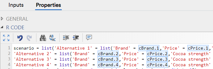
You can inspect the underlying code in the copied R Output by viewing Properties > R CODE in the Object Inspector. It will have a structure like the code below. In this example:
- Lines 1 to 4 describe the scenario that is being simulated, with one row for each alternative, and all four alternatives grouped as a list within a scenario list.
- Looking at Alternative 1, we can see that the level for Brand is set to cBrand.1, with the blue shading telling us that this is the name of something else in the project. In this case, the something else is the control on the page where the user selects the level of the brand attribute.
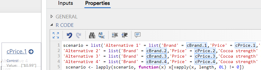
If you hover your mouse over any of the references to the controls, a box will appear to the left telling you the current selection. In the example below, we can see that the first alternative’s price has been set to “$0.99”.
Modifying the code
We can modify the code to insert other attribute levels. For example, if we replaced cPrice.1 with “$0.99”, we would get the same result as changing it in the price control. However, if we change the R code to “$0.99”, the code will no longer use the price control and will instead always use $0.99 as the price for alternative 1.
The code below is a modification of the code above, but it computes the demand curve. The key aspects of the code are:
- Lines 1 to 4 are identical to those that have been automatically created by the simulator bar changing the alternative list parameters to c.
- You can copy and modify Lines 5 to 13 as described in the remaining steps.
- The prices for the simulator are in line 5.
- In lines 10 and 11 replace “Alternative 3” with the name of the alternative that you are wanting to compute demand for. As shown in the screenshot below, in this case study, Hershey is Alternative 3.
- Replace hershey in line 13 with the name of the brand you are interested in.
Step 3: Creating the Visualization
You can now hook up your new table to a visualization from the Insert > Visualization menu. To create the area chart from my example above, click Insert > Visualization > Area and select your R table in the Inputs > DATA SOURCE > Output in ‘Pages’ drop-down in the Object Inspector.