
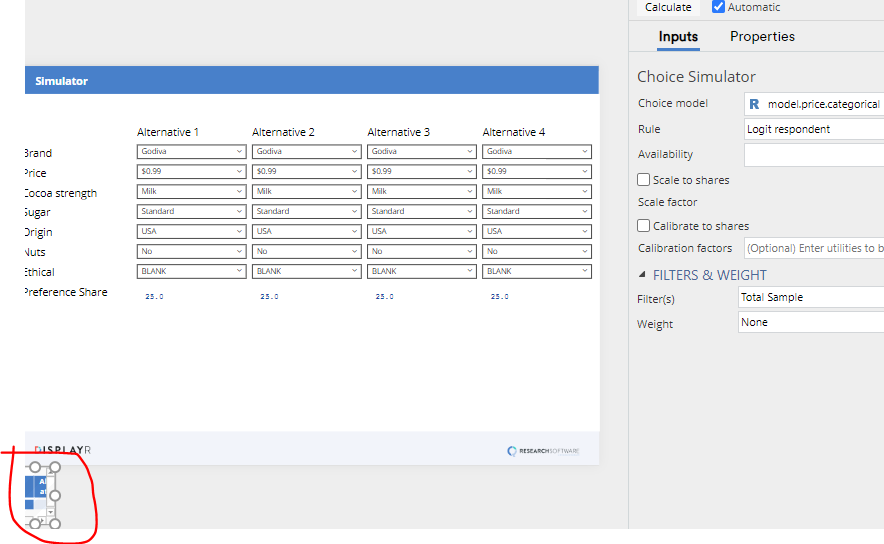
This post describes four methods for adjusting choice simulators from conjoint studies so that they better fit market share: change the choice rule, modify availability, tuning the scale factor, and calibration. The post assumes that you have first created a simulator, as per the instructions in Creating Online Conjoint Analysis Choice Simulators Using Displayr and have selected the calculations (see the image below).
Changing the choice rule
Choice simulators make assumptions about how to compute share given the estimated utilities. By default, Displayr computes preference share using utilities computed for each respondent. This is the typical way that preference is simulated in choice simulators. However, it is perhaps not the best method. When preferences are simulated using respondent utilities, we are implicitly assuming that the utilities are estimated without error. This assumption is not correct. As discussed in Performing Conjoint Analysis Calculations with HB Draws (Iterations), we can improve on our calculations by performing them using draws. This is theoretically better as it takes uncertainty into account. To do this we need to:
- Modify our choice model so that it saves the draws: set Inputs > SIMULATION > Iterations saved per individual to, say, 100. This will cause the model to be re-run
- Click on the calculations (see the screen shot above).
- In the object inspector on the right of the screen, change Rule from Logit respondent to Logit draw.
There are other rules. Rather than using the inverse logit assumption when computing preference shares, we can instead assume that the respondent chooses the alternative with the highest utility (First choice respondent) or that for each draw, the alternative with the highest utility is chosen (First choice draw). And, if you click Properties > R CODE you can edit the underlying code to implement more exotic rules (e.g., assume that people will only choose from the three most preferred options).
While you can modify these rules, it is recommended that you only use Logit draw or Logit respondent. The other rules, such as First choice respondent are only provided so that users who already use them in other programs have the ability to so in Displayr. The Logit draw rule is the actual rule that is explicitly assumed when the utilities are estimated, so if you use another rule, you are doing something that is inconsistent with the data and the utilities. Logit respondent is the most widely used rule largely because it is computationally easy; its widespread use suggests that it is acceptable.
Availability
Conjoint simulators assume that all the brands are equally available to all the respondents. However, in reality this assumption is unlikely. Some alternatives may not be distributed in some markets. Some may be available only in larger chains. Some may have really poor awareness levels. Some may have poor shelf placement.
The simplest way to deal with differences in availability is to create separate simulators for different markets and only include the alternatives in those markets in the simulators. A shortcut way of doing this for more technical users is to copy the calculations box multiple times, filtering each separately to each market, modifying the source code to remove alternatives, and then calculating the market share as the weighted sum of each of the separate market simulators.
Another approach is to factor in knowledge at the respondent level. We can incorporate this into a simulator by creating an R Output containing a matrix, where each row corresponds to a respondent, each column to one of the alternatives, with TRUE and FALSE indicating which alternative is available to which respondent. This is then selected in Availability in the object inspector.
For example, consider the situation where there is a data set of 403 respondents, we have four alternatives, and we wish to make the second alternative unavailable in Texas. We would do this as follows:
- Insert > R Output
- Paste in the code below
- Click on the calculations (i.e., see the top of this post)
- Set Availability to availability
The same approach can also be used to specify distribution in terms of percentages. The code below will generate availabilities such that the first alternative has a 50% distribution, the second 95%, the third 30%, and the fourth 100%.
When using randomness to take distribution into account, two additional things to consider are:
- Are there correlations between the distributions? For example, if small brands tend to not appear in the same stores, then simulating availability with a negative correlation between the availability of the smaller brands may be advisable.
- Simulation noise. This can be addressed by:
- Copying the calculations multiple times.
- Having a separate availability matrix for each, modifying the set.seed code in each (e.g., set.seed(1224) will generate a completely different set of random TRUEs and FALSEs).
- Calculating share as the average across the simulations.
More exotic modifications of distribution are possible by accessing the source code and using the offset parameter, as shown below.
Tuning the scale factor
Answering conjoint questions is boring. People make mistakes. We can be lazy and careless shoppers. We make mistakes. A basic conjoint simulator assumes that we make mistakes at the same rate in the real world as occurs when we fill in conjoint questionnaires. However, we can tune conjoint simulators so that they assume a different level of noise. The jargon for this is we can “tune” the scale factor.
The scale factor can be manually modified by clicking on the calculation and entering a value into the Scale factor field in the object inspector. The default value is 1. The higher the value, the less noise you are using in the simulation. As the scale factor approaches infinity, we end up getting the same results as when using a first choice rule. When the scale scale factor is 0, we assume each alternative is equally popular (assuming there are no availability effects).
You can automatically calculate the scale factor that best predicts known market shares as follows:
- Click on the calculations (i.e., see the top of this post).
- Click Scale to shares in the object inspector.
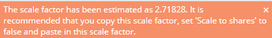
- Type in the shares of the alternatives in the Shares field as proportions (e.g., .26, .16, .12, .46). You will then see a message like the one shown below, showing the estimated scale factor.
- Using your mouse, select the number, right-click and select Copy.
- Uncheck Scale to shares.
- Click into Scale factor, right-click and select Paste.
Calibrating to market share
Calibration to market share involves modifying the utility of the alternative in such a way that the share predictions exactly match market share. This is more controversial than the other adjustments discussed in this post.
The main argument against calibration is that if the simulator inaccurately predicts current market share, all its predictions are likely inaccurate, so calibration is just making something inaccurate appear to be accurate, and thus is deceptive.
There are two counter arguments to this:
- The simulator is likely the best tool available, and by calibrating it you ensure that the base case matches the current market, making it easier for people to interpret the results.
- Calibration can be theoretically justified in the situation where important attributes have not been included in the study. For example, let’s say we were simulating preference for cola, and and we had only included the attributes of brand and price in the study. If there were important differences in the packaging of the brands, then this is a limitation of the study that could be addressed by calibration (provided that the respondents would not have inferred the packaging from the brand).
To calibrate a simulator:
- Click on the calculations (i.e., see the top of this post).
- Click Calibrate to shares in the object inspector.
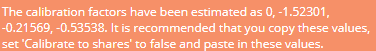
- Type in the shares of the alternatives in the Shares field as proportions (e.g., .26, .16, .12, .46). You will then see a message like the one shown below, showing the estimated scale factor..
- Using your mouse, select the numbers, right-click and select Copy.
- Uncheck Calibrate to shares.
- Click into Calibration factor, right-click and select Paste.
Do these four methods in order
In general, its advisable to apply these four adjustments in the order described in this post. In particular, availability should always be applied prior to scaling and calibration, and scaling prior to calibration.