
Conjoint analysis, and choice modeling in general, is super-powerful. It allows us to make predictions about the future. However, if the models are poor, the resulting forecasts will be wrong. This post walks through the 7 stages involved in checking a choice model.
The ‘hygiene test’: checking for convergence
Most modern conjoint analyses are estimated using hierarchical Bayes (HB). HB works by starting with an initial guess, and then continually improving on that guess. Each attempt at improving is called an iteration. Most choice modeling software stops after a pre-specified number of iterations have been completed. Sometimes this is too early, and more iterations are needed before the model can be safely relied upon. The technical term for when enough iterations have been achieved is that the model has achieved convergence.
When a model has not converged, the fix is to increase the number of iterations, also known as draws, until convergence is achieved.
Just as with hygiene tests in food safety, a lack of convergence is no guarantee that the model is unsafe. Food prepared in the most unhygienic situations can be safe if you have the right bacteria in your gut. Similarly, conjoint models that have not converged can give you the right answer. For this reason, it is very common for people to conduct conjoint studies without ever checking hygiene. Of course, just like with cooking, poor hygiene can have devastating consequences, so why take the risk?
Modern choice software, such as Displayr, automatically performs such hygiene tests and provides warnings where the model has not converged. However, all hierarchical Bayes software can produce, or be used to compute, the relevant diagnostics for checking for convergence: the Gelman-Rubin statistic (Rhat), examining the effective sample size, and viewing trace plots. Please see “Checking Convergence When Using Hierarchical Bayes for Conjoint Analysis“.
The ‘smell test’: checking the distributions of the coefficients
Once it is believed that the model has converged, the next step is to inspect the distribution of the estimated utilities (coefficients). This is the “smell test”. If something is rotten, there is a good chance of discovering it at this stage. Unlike the hygiene test, it is super powerful.
The output below shows the distributions of utilities for the first two attributes of a study of the chocolate market. The experimental design showed four alternatives in each choice question. The first attribute is Alternative, where a 1 indicates that the alternative was the left of the four shown to the respondents, the 2 is the second alternative, and so on.
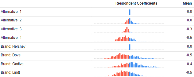
Alternative 1 has a mean of 0 and a single blue column in its histogram, indicating no variation. As discussed in Choice Modeling: The Basics, choice models start with an assumption that one of the attribute levels has a utility of 0, and thus this is an assumption rather than a result. Looking at alternative 2, we can see its mean is the same as alternative 1’s, which makes sense. There is a bit of variation between the respondents, which is consistent with there being a bit of noise in the data. For alternative 3 and 4, however, we see that they have lower means, suggesting that people were consistently less likely to choose these options. This is disappointing, as it suggests that people were not carefully examining the alternatives. The good news is we can take this effect out of the model at simulation time (by removing this attribute from the simulations, or, by using its average value if there is ‘none of these’ alternative). If you are using software that does not produce utilities for alternatives, which are also known as alternative specific constants, make sure that you include them manually as an extra attribute, as it is one of those rare things that is both easy to check and easy to fix.
Looking at the averages for the four brands, again the first brand has been pegged at 0 for all respondents, and the other results are relative to this. We can see that the means for Dove and Lindt are less than 0, so they are on average less preferred than Hershey (all else being equal), whereas Godiva has a higher average preference. For each of the brands there is quite a lot of variation (fortunately a lot more than for the alternative), suggesting that people differ a lot in their preferences.
The output below shows the utilities for the remaining attributes. For the price attribute, the first price level is set to 0 for everybody. We see that progressively higher prices have lower average levels of preference, but there is some variability about this. This is in line with common sense, and good news, as it shows that the data smells OK.
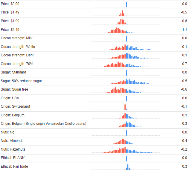
The data on cocoa strength, sugar, origin, and nuts, are not so useful from a smell test perspective. As with brand, there is no obvious way of checking if it smells good. We can, nevertheless, draw some broad conclusions.
- The 70% Cocoa is least preferred on average, but is divisive. On average people want a reduction in sugar, but most do not want sugar free.
- Origin is relatively unimportant. There is little difference in the means and not much variation in the preference.
- On average people prefer no nuts, but there is variation in preference, particularly with regards to hazelnuts.
- We should expect all but non-contrarians to prefer free trade. We do see this, but also see little variation, telling us that it is an unimportant attribute.
No random choosers (RLH statistic)
Choice modeling questions can be a bit boring. When bored, some respondents will select options without taking the time to evaluate them with care. Fortunately, this is easy to detect with a choice model: we look at how well the model predicts a person’s actual choices. The simplest way to do this is to count up the number of correct choices. However, there is a better way, which is to:
- Fit a choice model without an attribute for alternative (i.e., without estimating alternative specific constants). The reason that this is important is that if a person has chosen option 3 every time, a model with an attribute of alternative may predict their choices very well. Where the model includes none of these alternatives, the trick is to merge together the levels of the attributes other than ‘none of these’. In a labeled choice experiment, you need to skip this step and proceed with the model with the attribute for alternatives.
- For each question, compute the probability that the person chooses the option that they choose.
- Multiply the probabilities together. For example, in a study involving four questions, if a person chooses an option that the model predicted they had a 0.4 probability of choosing, and their choices in the remaining three questions had probabilities of 0.2, 0.4, and 0.3 respectively, then the overall probability is 0.0096. This is technically known as the person’s likelihood.
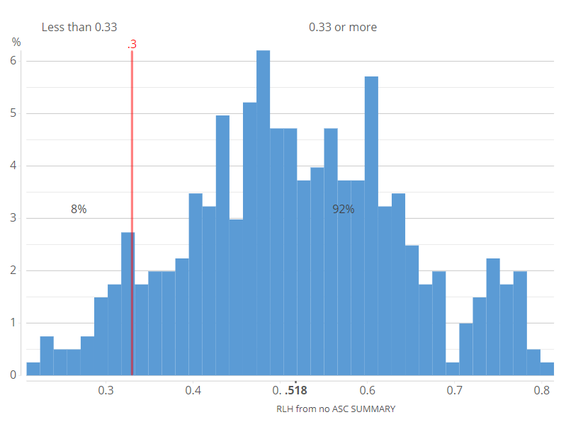
- Compute likelihood^(1/k), where k is the number of questions. In this example, the result is 0.31. The value is known as the root likelihood (RLH). It is better than just looking at the percentage of the choices that the the model predicts correctly, as it rewards situations where the model was close and penalizes situations where the model was massively wrong. Note that the RLH value of 0.31 is close to the mean of the values (technically, it is the geometric mean).
- Plot the RLH statistics for each person and determine a cutoff point, re-estimating the model using only people with RLH statistics above the cutoff value. In the chocolate study from earlier, we gave people a choice of four options, which tells us that the cutoff point needs to be at least 1/4 = 0.25. However, hierarchical Bayes models tend to overfit conjoint analysis data, so a higher cutoff is prudent. The histogram below suggests that there are a clump of people at around 0.33, which perhaps represents random choosers, but there is no easy way to be sure (if your data contains information on time taken to complete questions, this can also be taken into account).
Rational choosing
Random choosing is a pretty low threshold for quality of data. A higher threshold is to check that the data exhibits “rationality”, where here the term “rational” is a term of art from economics, which essentially means that the person is making choices in a way that is consistent with their self interests. Working out if choices in conjoint questionnaires are rational is an ongoing area of research, and lots of work shows that they are often not rational (e.g., irrelevant information shown earlier in a questionnaire can influence choices). Nevertheless, in most studies it is possible to draw some conclusions regarding what constitutes irrationality. Among the people that did not seem to be randomly choosing, 6% had data indicating they preferred to pay $2.49 to $0.99.
While it may be tempting to exclude these 6%, it would be premature. Inevitably some people will find price relatively unimportant, and for these people there will be uncertainty about their preference for price. A more rigorous analysis is to only exclude people where it is highly likely they have ignored price. Such an analysis leads to only excluding 1 person (0.3% of the sample). In the post Performing Conjoint Analysis Calculations with HB Draws (Iterations), I describe the basic logic of such an analysis.
Cross-validation
A basic metric for any choice model is its predictive accuracy. The chocolate study has a predictive accuracy of 99.4% after removing the respondents with poor data. This sounds too good to be true, and it is too good. This predictive accuracy is computed by checking to see how well the model predicts the data used to fit the model.
A more informative approach to assessing predictive accuracy is to check the model’s performance on data not used to fit the model (this is called cross-validation). Where the choice model is estimated using an experiment, say asking people 6 questions each, predictive accuracy is assessed by estimating a model with one question randomly selected not to be used when fitting the model, and then seeing how well the model predicts these choices. In the case of the chocolate study, when this is done the predictive accuracy drops markedly to 55.4%. As the study involved four alternatives, this is well above chance (chance being 25% predictive accuracy).
Checking that the utilities are appropriately correlated with other data
All else being equal, we should expect that the utilities computed for each person are correlated with other things that we know about them. In the chocolate study this occurs, with diabetics having higher utility for sugar-free chocolate, and people with higher incomes not having as low utility for higher prices as did those with lower incomes.
A word to the wise: avoid using gut feel and prejudice. For example, it is pretty common for marketers to have strong beliefs about the demographic profiles of different brands’ buyers (e.g., Hershey’s will be bought by poorer people than Godiva). It is often the case that such beliefs are not based on solid data. It is therefore a mistake to conclude a choice model is bad if it does not align with beliefs, without checking the quality of the beliefs.
Ability to predict historic market performance
While the goal of a choice model is to make predictions about the future, they can also be used to make predictions about the past. For example, if a choice model collects price data, it can be used to predict the historic impact of changes in price. If the predictions of history are poor, it is suggestive that the model will also not predict the future well. You can find out more about this in 12 Techniques for Increasing the Accuracy of Forecasts from Choice Experiments.
All the calculations described in this post can be reviewed in this Displayr document.