


There are a number of different approaches to calculating relative importance analysis including Relative Weights and Shapley Regression as described here and here. In this blog post I briefly describe how to use an alternative method, Partial Least Squares, in R. Because it effectively compresses the data before regression, PLS is particularly useful when the number of predictor variables is more than the number of observations.
What are Partial Least Squares?
Partial Least Squares sometimes known as Partial Least Square regression or PLS is a dimension reduction technique with some similarity to principal component analysis. The predictor variables are mapped to a smaller set of variables, and within that smaller space we perform a regression against the outcome variable. In Principal Component Analysis the dimension reduction procedure ignores the outcome variable. However PLS aims to choose new mapped variables that maximally explain the outcome variable.
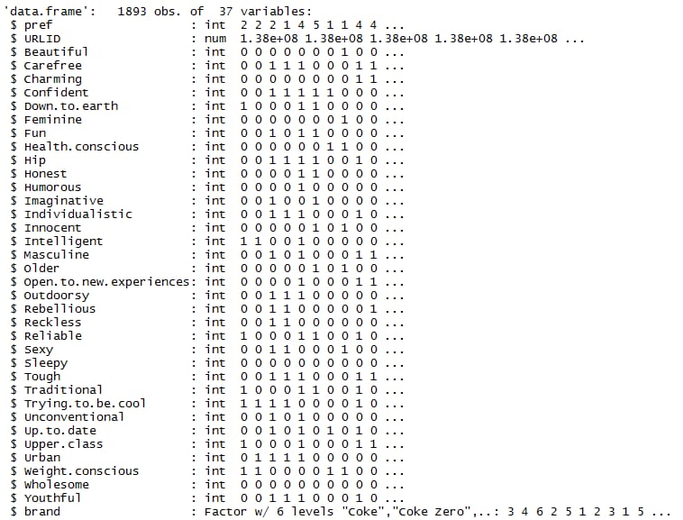
To get started I’ll import some data into R and examine it with the following few lines of code:
cola.url = "http://wiki.q-researchsoftware.com/images/d/db/Stacked_colas.csv"
colas = read.csv(cola.url)
str(colas)
The output below show 37 variables. I am going to predict pref, the strength of a respondent’s preference for a brand on a scale from 1 to 5. To do this I’ll use the 34 binary predictor variables that indicate whether the person perceives the brand to have a particular characteristic.
Using Partial Least Squares in R
The next step is to remove unwanted variables and then build a model. Cross validation is used to find the optimal number of retained dimensions. Then the model is rebuilt with this optimal number of dimensions. This is all contained in the R code below.
colas = subset(colas, select = -c(URLID, brand))

library(pls)
pls.model = plsr(pref ~ ., data = colas, validation = "CV")

# Find the number of dimensions with lowest cross validation error
cv = RMSEP(pls.model)
best.dims = which.min(cv$val[estimate = "adjCV", , ]) - 1

# Rerun the model
pls.model = plsr(pref ~ ., data = colas, ncomp = best.dims)
Producing the Output
Finally, we extract the useful information and format the output.
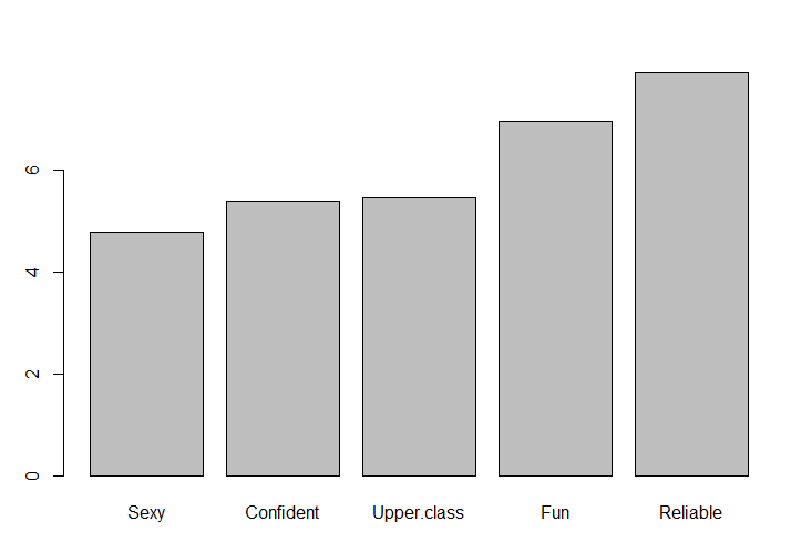
coefficients = coef(pls.model)
sum.coef = sum(sapply(coefficients, abs))
coefficients = coefficients * 100 / sum.coef
coefficients = sort(coefficients[, 1 , 1])
barplot(tail(coefficients, 5))
The regression coefficients are normalized so their absolute sum is 100 and the result is sorted.
The results below show that Reliable and Fun are positive predictors of preference. You could run the code barplot(head(coefficients, 5)) to see that at the other end of the scale Unconventional and Sleepy are negative predictors.
TRY IT OUT
Displayr is a data science platform providing analytics, visualization and the full power of R. You can perform this analysis for yourself in Displayr.