
A previous blog post described a smart way of computing the Net Promoter Score by recoding. The idea was to recode NPS ratings from 0 to 10 into three numeric values: -100 for the Detractors (respondents who gave a rating from 0 to 6), 0 for the Neutrals (7 or 8) and 100 for the Promoters (9 or 10). The NPS was obtained from the average of the recoded ratings. The post briefly mentioned that statistical testing could be conducted on the NPS by treating it as an average but did not go into the details of how or why this is possible In this blog post I discuss the statistical testing of NPS, and derive expressions for estimating the standard error of NPS.
Statistical testing is essential when analyzing customer feedback data. It allows you to separate signal from noise, and test whether your results are truly meaningful.
The problem and the solution
Having computed the NPS, it is common to want to determine if it is significant from zero or if it is different from another NPS. But how should this be done? The NPS is computed as a difference between percentages, and while there are lots of statistical tests for comparing percentages, there are none for comparing differences in correlated percentages (they are correlated in that if you have more promoters you will likely have less detractors, and vice versa).
Fortunately, it turns out that even though the NPS does not follow a normal distribution, we can test using standard t-tests. The use of the t-test is valid as NPS approaches normality as the sample size increases (via the central limit theorem) and the t-test is highly robust to deviations from normality.
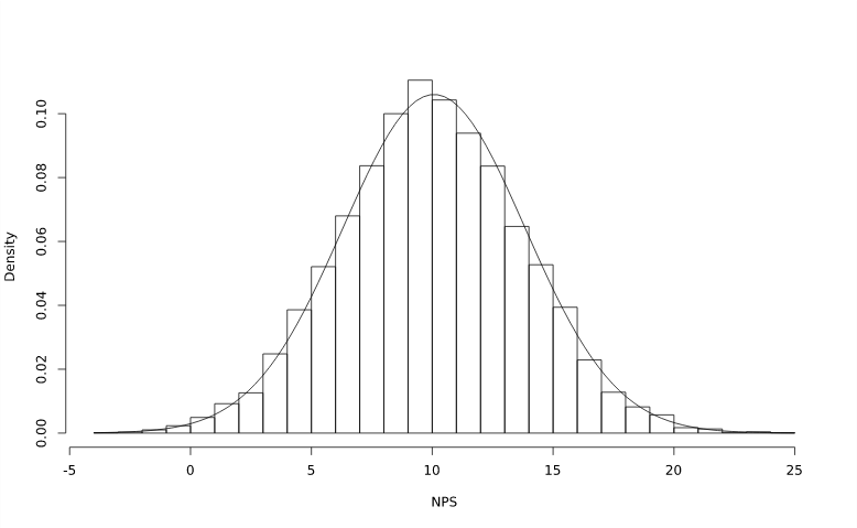
The histogram at the top of this post was generated from 10,000 simulations of a 500-respondent survey in which the probability of a respondent being a Promoter was 40%, and the probability of a respondent being a Detractor was 30%. A normal distribution (that was fit to the data) was overlaid on top of the histogram, and it shows how close NPS is to being normally distributed even with a moderately-sized sample.
Computing t-tests
To conduct a t-test, the standard error of the NPS first needs to be estimated (see the following sections on how to do this). The t-statistic to test if the NPS is significant from  (the null hypothesis is
  ) is
) is
![\[ t=\frac{\textrm{NPS}-\mu_0}{SE_{\textrm{\tiny{NPS}}}} \]](https://www.displayr.com/wp-content/ql-cache/quicklatex.com-2ef2c5581b70ede932f908171bbaf7fe_l3.png "Rendered by QuickLaTeX.com")
where the degrees of freedom to use in this t-test is  . To test significance from zero, set
  . The t-statistic for comparing two NPS values (the null hypothesis is
  ) is
) is
![\[ t=\frac{\textrm{NPS}_1-\textrm{NPS}_2}{\sqrt{SE_1^2+SE_2^2}} \]](https://www.displayr.com/wp-content/ql-cache/quicklatex.com-a2edb55bb0ac6e5288e4ebb013ea85f9_l3.png "Rendered by QuickLaTeX.com")
where the degrees of freedom to use in this t-test is
![\[ \frac{\left(SE_1^2+SE_2^2\right)^2}{SE_1^4/(n_1-1)+SE_2^4/(n_2-1)}. \]](https://www.displayr.com/wp-content/ql-cache/quicklatex.com-b203541171bc6772e4ca31952656e25e_l3.png "Rendered by QuickLaTeX.com")
where  and
and  denote the sample sizes for
  and
and  respectively.
Deriving the NPS standard error
Let the total number of respondents be  and let the random variables
  ,
,  and
and  denote the number of Detractors, Neutrals and Promoters respectively, so that
  . The NPS score is calculated using the formula
  . The standard error of the NPS score is
![\[ SE_{\textrm{\tiny{NPS}}}=\textrm{SD}\left(\frac{100(x_A-x_D)}n\right)=\sqrt{\textrm{Var}\left(\frac{100(x_A-x_D)}n\right)}. \]](https://www.displayr.com/wp-content/ql-cache/quicklatex.com-c67badbea6bbecc7b7ecbbcaf94a304a_l3.png "Rendered by QuickLaTeX.com")
Using the properties of the variance of random variables, this becomes
(1) ![\[ SE_{\textrm{\tiny{NPS}}}=100\sqrt{\frac{\textrm{Var}(x_A)}{n^2}+\frac{\textrm{Var}(x_D)}{n^2}-\frac{2\textrm{Cov}(x_A,x_D)}{n^2}}. \]](https://www.displayr.com/wp-content/ql-cache/quicklatex.com-f984c251b42447d2019de647d35895f2_l3.png "Rendered by QuickLaTeX.com")
If the probabilities of these respondents being Detractors, Neutrals and Promoters are  ,
,  and
and  respectively, the vector of random variables
  follows a multinomial distribution. The variance and covariance of such variables are
![\[ \textrm{Var}(x_A)=np_A(1-p_A),\qquad\textrm{Var}(x_D)=np_D(1-p_D),\qquad\textrm{Cov}(x_A,x_D)=-np_Ap_D. \]](https://www.displayr.com/wp-content/ql-cache/quicklatex.com-0df62f1c2f67314135f2e889988e987b_l3.png "Rendered by QuickLaTeX.com")
Plugging this back into (1), we get
(2) ![\[ SE_{\textrm{\tiny{NPS}}}=100\sqrt{\frac{p_A(1-p_A)}n+\frac{p_D(1-p_D)}n+\frac{2p_Ap_D}n}=100\sqrt{\frac{p_A+p_D-(p_A-p_D)^2}n}. \]](https://www.displayr.com/wp-content/ql-cache/quicklatex.com-49709c23ce80255be03b4700cedf2f49_l3.png "Rendered by QuickLaTeX.com")
This is an exact formula for the standard error which relies on knowing and . In practice, we do not know the values of these but we can estimate them from the number of Detractors and Promoters:
![\[ \widehat p_A=\frac{x_A}n,\qquad\widehat p_D=\frac{x_D}n. \]](https://www.displayr.com/wp-content/ql-cache/quicklatex.com-651a548d2888e73e2d2e5627857cb03e_l3.png "Rendered by QuickLaTeX.com")
Using this to replace and in (2), a sample estimate of the standard error is therefore
(3) ![\[ \widehat{SE}_{\textrm{\tiny{NPS}}}=\frac{100}n\sqrt{x_A+x_D-\frac{(x_A-x_D)^2}n}. \]](https://www.displayr.com/wp-content/ql-cache/quicklatex.com-06e27ad7d51616c3985cdacab7089771_l3.png "Rendered by QuickLaTeX.com")
NPS standard error from the average of recoded ratings
Let  denote the set of recoded ratings. The NPS can be computed as sample mean
  . An estimate of the standard error of is
![\[ \widehat{SE}_{\overline z}=\frac{\textrm{SD}(Z)}{\sqrt{n}}=\sqrt{\frac1{n(n-1)}\sum_{i=1}^n(z_i-\overline z)^2}=\sqrt{\frac1{n(n-1)}\sum_{i=1}^n\left(z_i^2-2z_i\overline z+\overline z^2\right)}. \]](https://www.displayr.com/wp-content/ql-cache/quicklatex.com-ab42989f704426bff036ac30b31f9212_l3.png "Rendered by QuickLaTeX.com")
Since
![\[ \overline z=\frac{100(x_A-x_D)}n,\qquad\sum_{i=1}^nz_i=100(x_A-x_D),\qquad\sum_{i=1}^nz_i^2=10000(x_A+x_D), \]](https://www.displayr.com/wp-content/ql-cache/quicklatex.com-5dfebecbe03daf2d17518b633858e0b4_l3.png "Rendered by QuickLaTeX.com")
the standard error of becomes
(4) ![\[ \widehat{SE}_{\overline z}=\frac{100}{\sqrt{n(n-1)}}\sqrt{x_A+x_D-\frac{(x_A-x_D)^2}n}. \]](https://www.displayr.com/wp-content/ql-cache/quicklatex.com-1e2c04a222f991f0a3cf5e927022c114_l3.png "Rendered by QuickLaTeX.com")
Comparing (3) and (4), we can see that the two expressions are the same except that in (3) has been replaced with in (4) due to Bessel’s correction for bias. In my opinion, (4) is the better formula to use since bias would have been introduced when substituting in  and
and  to obtain (3).
Learn how to statistically test Net Promoter Score in Displayr
Summary
I have shown how to setup t-tests for NPS and discussed why this approach is valid. Two ways of estimating the standard error for NPS were derived, where the approach based on averaging recoded ratings was deemed superior. Advanced Net Promoter Score analysis software, like Displayr, run a lot of statistical tests behind the scenes, taking the mathematics off your hands. However, it’s always handy to know how your software is operating under the hood.