These include both global methods, which involve fitting a regression over the whole time series; and more flexible local methods, where we relax the constraint by a single parametric function. Further details about how to construct estimated smooths in R can be found here.
1. Global trends over time
i. Linear
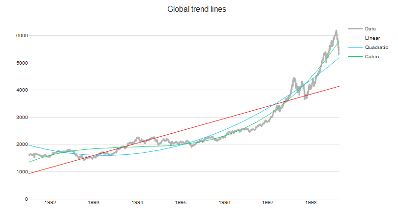
One of the simplest methods to identify trends is to fit the time series to the linear regression model.
ii. Quadratic
For more flexibility, we can also fit the time series to a quadratic expression — that is, we use linear regression with the expanded basis functions (predictors) 1, x, x2.
iii. Polynomial
If the linear model is not flexible enough, it can be useful to try a higher-order polynomial. In practice, polynomials of degrees higher than three are rarely used. As demonstrated in the example below, changing from quadratic and cubic trend lines does not always significantly improve the goodness of fit.
2. Local smoothers
The first three approaches assume that the time series follows a single trend. Often, we want to relax this assumption. For example, we do not want variation at the beginning of the time-series to affect estimates near the end of the time series. In the following section, we demonstrate the use of local smoothers using the Nile data set (included in R's built in data sets). It contains measurements of the annual river flow of the Nile over 100 years and is less regular than the data set used in first example.
i. Moving averages
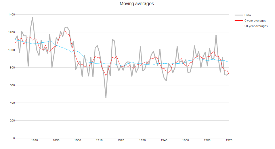
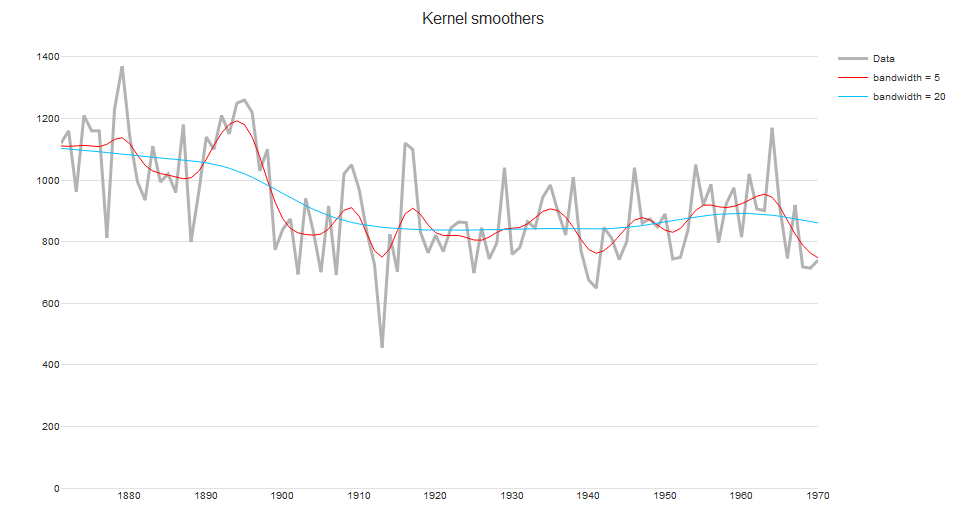
The easiest local smoother to grasp intuitively is the moving average (or running mean) smoother. It consists of taking the mean of a fixed number of nearby points. As we only use nearby points, adding new data to the end of the time series does not change estimated values of historical results. Even with this simple method we see that the question of how to choose the neighborhood is crucial for local smoothers. Increasing the bandwidth from 5 to 20 suggests that there is a gradual decrease in annual river flow from 1890 to 1905, instead of a sharp decrease at around 1900.
ii. Running line
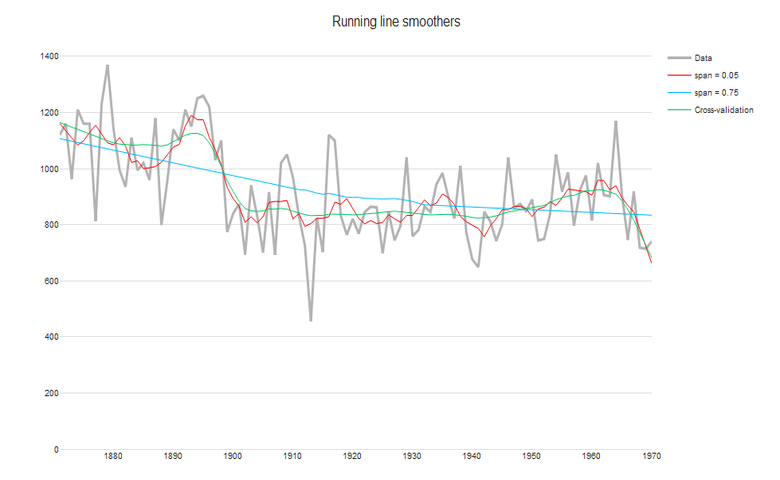
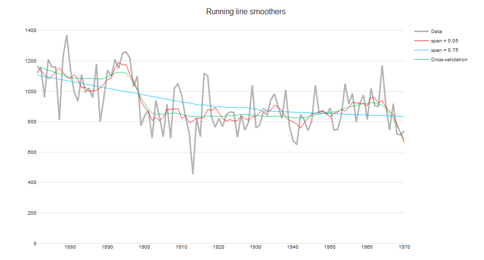
The running-line smoother reduces this bias by fitting a linear regression in a local neighborhood of the target value xi. A popular algorithm using the running line smoother is Friedman’s super-smoother, which uses cross-validation to find the best span. As seen in the plot below, the Friedman's super-smoother with the cross-validated span is able to detect the sharp decrease in annual river flow at around 1900.
iii. Kernel smoothers
An alternative approach to specifying a neighborhood is to decrease weights further away from the target value. In the figure below, we see that the continuous Gaussian kernel gives a smoother trend than a moving average or running-line smoother.
iv. Smoothing splines
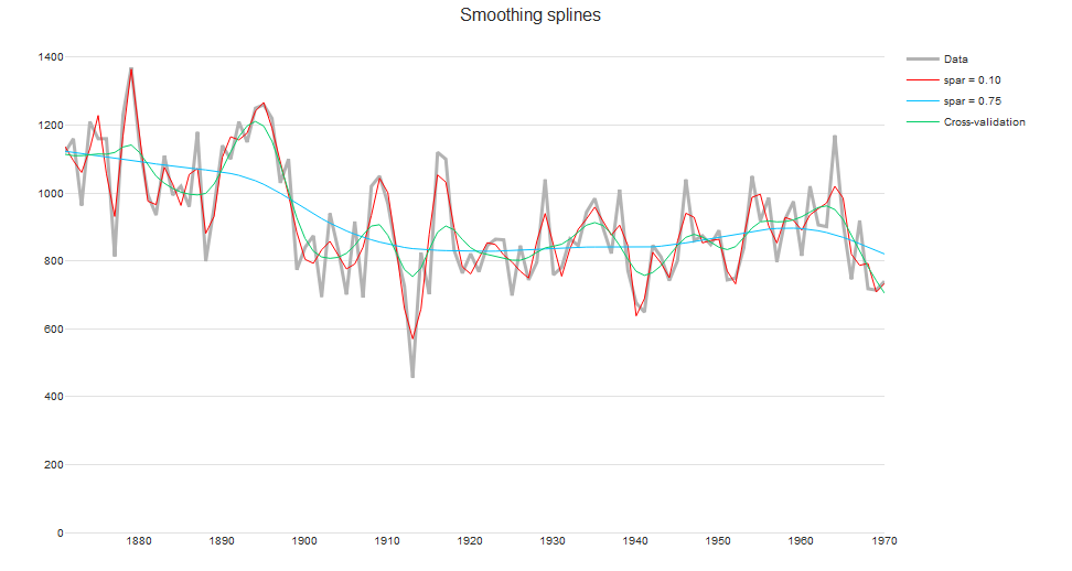
Splines consist of a piece-wise polynomial with pieces defined by a sequence of knots where the pieces join smoothly. It is most common to use cubic splines. Higher order polynomials can have erratic behavior at the boundaries of the domain.
The smoothing spline avoids the problem of over-fitting by using regularized regression. This involves minimizing a criterion that includes both a penalty for the least squares error and roughness penalty. Knots are initially placed at all of the data points. But the smoothing spline avoids over-fitting because the roughness penalty shrinks the coefficients of some of the basis functions towards zero. The smoothing parameter lambda controls the trade-off between goodness of fit and smoothness. It can be chosen by cross-validation.
v. LOESS
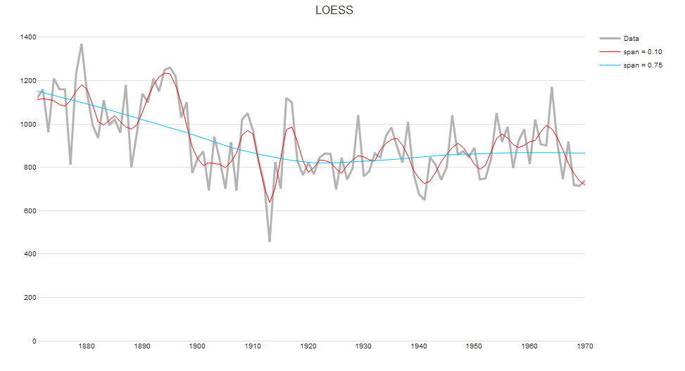
LOESS (locally estimated scatterplot smoother) combines local regression with kernels by using locally weighted polynomial regression (by default, quadratic regression with tri-cubic weights). It is one of the most frequently used smoothers because of its flexibility. However, unlike Friedman’s super smoother or the smoothing spline, LOESS does not use cross-validation to select a span.
Find out more about data visualizations here.

