A Comprehensive Guide to Cluster Analysis: Applications, Best Practices and Resources

Cluster analysis has a wide  range of applications in various fields, including marketing, biology, finance, and social sciences. For example, it can be used to identify genetic markers associated with specific diseases, to detect anomalies in financial transactions, and to classify social media users into different categories based on their interests and behaviors. It is commonly used in market research for segmenting customers into groups based on their buying behaviors. 

This page will provide a comprehensive guide to cluster analysis, covering the different techniques and algorithms used in the process, best practices for conducting cluster analysis on big data, common challenges and how to overcome them, and real-world case studies demonstrating the application of cluster analysis in practice.

Cluster analysis in 2023: Whether you are a researcher, data or insights analyst or consultant, it is important to have a tool that can aid in the clustering process. Try this cluster analysis template in Displayr.

Introduction to Cluster Analysis

Definition and purpose of cluster analysis

Cluster analysis is a statistical technique in which algorithms are used to group a set of objects or data points into groups based on their similarity.

The result of cluster analysis is a set of clusters, where each cluster is distinct from one another, and the objects or data points within each cluster are largely similar to each other.

The purpose of cluster analysis is to help reveal patterns and structures within a dataset that may provide insights into underlying relationships and associations.

 

Applications of cluster analysis

Cluster analysis has a huge range of applications across different fields and industries. Here are some common examples:

1. Market Segmentation: Cluster analysis is often used in marketing to segment customers into groups based on their buying behavior, demographics, or other characteristics. This information can be used to create targeted marketing campaigns or to develop new products that appeal to specific customer groups.
2. Image Processing: In image processing, cluster analysis is used to group pixels with similar properties together, allowing for the identification of objects and patterns in images.
3. Biology and Medicine: Cluster analysis is used in biology and medicine to identify genes associated with specific diseases or to group patients with similar clinical characteristics together. This can help with the diagnosis and treatment of diseases.
4. Social Network Analysis: In social network analysis, cluster analysis is used to group individuals with similar social connections and characteristics together, allowing for the identification of subgroups within a larger network.
5. Anomaly Detection: Cluster analysis can be used to detect anomalies in data, such as fraudulent financial transactions, unusual patterns in network traffic, or outliers in medical data.

Types of Cluster Analysis

There are several different types of cluster analysis as thousands of algorithms have been developed that attempt various ways to group objects into clusters. This guide will cover some of the main ones:

Hierarchical clustering

Hierarchical clustering is a method that creates a hierarchy of clusters by recursively splitting or merging them based on their similarities. This type of clustering can be either agglomerative (starting with single data points and merging them into clusters) or divisive (starting with all data points in a single cluster and dividing them into smaller ones). However, divisive hierarchical clustering is rarely performed in practice.

Instead, it is far more common to perform agglomerative hierarchical clustering where each observation is treated as a separate cluster and then the following steps are repeated:

1. Identify the two cluster that are the most similar
2. Merge those two clusters

This process is continued until all the clusters are merged together.

 

K-means clustering

K-means clustering is a method that groups data points into a predetermined number (k) of clusters based on their distances to the centroid of each cluster. This is an iterative algorithm that aims to minimize the sum of squared distances between data points and their assigned cluster centroids.

K-means cluster analysis follows these steps:

1. Specify the number of clusters. This is referred to as k. Normally, researchers will conduct k-means several times, exploring different numbers of clusters as the starting point.
2. Allocate objects to clusters. The most straightforward approach here is to randomly assign objects to clusters.
3. Compute cluster means. For each cluster, the average value is computed for each of the variables.
4. Allocate each observation to the closest cluster center.
5. Repeat steps 3 and 4 until the solution converges.

 

Model-based clustering

Model based clustering is a method that assumes that the data points within each cluster follow a particular probability distribution. This type of clustering is often used when the underlying data distribution is not well-known or when the data contains noise or outliers.

 

Density-based clustering

Density-based clustering is a method that groups data points together based on their density within a defined radius or distance threshold. This type of clustering is useful for identifying clusters with irregular shapes or clusters that are widely separated.

 

Fuzzy Clustering

Fuzzy clustering is a method that assigns each data point a membership score for each cluster, rather than a binary membership value. This type of clustering is useful when data points can belong to more than one cluster simultaneously or when there is uncertainty about which cluster a data point belongs to.

Data Preparation for Cluster Analysis

There are some important steps to consider when preparing your data for cluster analysis.

Data cleaning and transformation

Before performing cluster analysis, it's important to ensure that the data is clean and free from errors. This may involve removing missing values, outliers, or duplicates.

You may also need to get your data in the right format. Typically, cluster analysis is performed on a table of raw data, where each row represents an object and the columns represent quantitative characteristics of the objects. These quantitative characteristics are called clustering variables.

For example, in market segmentation, where k-means is used to find groups of consumers with similar needs, each object is a person and each variable is commonly a rating of how important various things are to consumers (e.g., quality, price, customer service, convenience).

Cluster analysis can also be performed using data in a distance matrix.

Handling missing values

Most cluster analysis software or algorithms will not work with missing values in the data, so you will want to handle any missing values immediately.

There are five main options for dealing with missing data when using cluster analysis. They are: complete case analysis, complete case analysis followed by nearest-neighbor assignment for partial data, partial data cluster analysis, replacing missing values or incomplete data with means, imputation.

Complete case analysis

Complete case analysis involves using only data points with complete information in the analysis - any data points that contain missing values are removed.

However, this approach assumes that the data is Missing Completely At Random and that the missing values have the same characteristics as the cases with complete data. Unfortunately, this is almost never true in reality. By removing data with missing values, the size of the dataset is reduced and may result in problems such as a bias in the clustering results.

Complete case analysis followed by nearest-neighbor assignment for partial data

The complete case analysis followed by nearest assignments for partial data follows the same approach as complete case analysis but with the added step of assigning the remaining observations to the closest cluster based on the available data.

Partial data cluster analysis

Partial data cluster analysis involves grouping observations together based on the data they have in common.

Replacing missing values with means

Another way of dealing with missing data is to replace missing values with the mean value of that variable.

Imputation

Another approach is to impute or estimate the missing values. One form of imputation is the same as the method above – mean imputation. But there are other forms such as regression imputation (using regression models to predict missing values), or k-nearest neighbor imputation (using the values of the nearest neighbors to estimate missing values).

Scaling and normalization

If the variables in the data have different scales, it's important to normalize or standardize them so that they have similar ranges. This can help prevent variables with larger scales from dominating the clustering process.

Although, scaling, normalization and standardization are related terms, they do not mean the same thing. Normalization refers to the process of changing the values of numeric columns in the dataset to a common scale. Standardization refers to changing the feature values, while the shape of the distribution doesn’t change.

Feature selection

Depending on the complexity of the data, it may be necessary to select a subset of the most relevant features to include in the clustering analysis. This can help reduce noise and improve the quality of the clustering results.

Choosing the Right Number of Clusters

Before performing the actual clustering, it's important to determine the optimal number of clusters. This can be done using a variety of methods, such as the elbow method, silhouette analysis, or gap statistic.

Elbow method

The elbow method is one of the most popular approaches for determining the optimal number of clusters in a clustering analysis. The elbow method involves plotting the within-cluster sum of squares (WSS) against the number of clusters, and selecting the number of clusters at the "elbow" or bend in the plot.

The within-cluster sum of squares is a measure of the sum of the squared distances between each data point and its assigned cluster centroid. The goal of clustering analysis is to minimize the within-cluster sum of squares, and the plot of the WSS against the number of clusters can help identify the optimal number of clusters.

To apply the elbow method, the following steps can be followed:

1. Perform clustering analysis using a range of different numbers of clusters, for example, from 1 to 10.
2. Calculate the within-cluster sum of squares (WSS) for each clustering solution.
3. Plot the WSS against the number of clusters.
4. Examine the plot and look for the "elbow" or bend in the curve. This is the point where adding more clusters does not significantly reduce the within-cluster sum of squares.
5. Select the number of clusters at the elbow point as the optimal number of clusters.

It's important to note that the elbow method is not always clear-cut, and the choice of the optimal number of clusters can be somewhat subjective. In addition, the elbow point may not always be visible in the plot, particularly if the data is complex or if there are multiple distinct clusters. Other methods, such as silhouette analysis or gap statistic, can also be used in conjunction with the elbow method to help determine the optimal number of clusters.

Silhouette analysis

Silhouette analysis is another technique you can use to evaluate the quality of your clustering results and determine the optimal number of clusters. provides a way to measure how well each data point fits into its assigned cluster and how distinct it is from the points in other clusters. The higher the silhouette score, the better the clustering results.

Here’s how to apply silhouette analysis:

1. Perform cluster analysis: Begin by applying a clustering algorithm, such as K-means or hierarchical clustering. Choose a range of possible cluster numbers, typically from 2 to a certain maximum value.
2. Compute silhouette coefficients: For each clustering result, calculate the silhouette coefficient for each data point. The silhouette coefficient for a particular data point is calculated as follows:
   1. Compute the average distance between the data point and all other points within the same cluster. This value is called the "intra-cluster distance" or "a(i)".
   2. Compute the average distance between the data point and all points in the nearest neighboring cluster. This value is called the "inter-cluster distance" or "b(i)".
   3. Calculate the silhouette coefficient for the data point using the formula: silhouette coefficient (s(i)) = (b(i) - a(i)) / max(a(i), b(i)).
3. Calculate the average silhouette score: Once you have the silhouette coefficient for each data point, compute the average silhouette score for each clustering result. The average silhouette score is the mean of all the silhouette coefficients in the dataset and provides an overall measure of the clustering quality.
4. Analyze the silhouette scores: Plot the average silhouette scores for different cluster numbers on a graph, with the number of clusters on the x-axis and the average silhouette score on the y-axis. Look for the cluster number that corresponds to the highest average silhouette score.
5. Select the optimal number of clusters: Based on the silhouette scores, choose the number of clusters that maximizes the average silhouette score. This indicates the clustering result with the best separation and coherence among the clusters.
6. Validate the chosen clusters: After selecting the optimal number of clusters, validate the clustering results using other evaluation metrics and domain knowledge to ensure they align with your understanding of the data.

Some data scientists and researchers consider the Silhouette method to be better than the Elbow method because you can use the Silhouette method to study the distance between your clusters and find outliers.

Gap statistic

The gap statistic is another method that can be used to determine the optimal number of clusters in cluster analysis. It compares the within-cluster dispersion of data points with their expected dispersion under null reference distributions. The idea is to identify the number of clusters where the gap statistic reaches its maximum value, indicating a good balance between compactness within clusters and separation between clusters.

Here's how you can use the gap statistic to find the optimal number of clusters:

1. Perform cluster analysis: Similar to silhouette analysis, start by applying a clustering algorithm (e.g., K-means) to your dataset. Specify a range of possible cluster numbers, typically from 2 to a maximum value.
2. Generate reference datasets: To estimate the expected dispersion under null reference distributions, generate reference datasets. These datasets should have the same feature dimensions as your original data but should be generated from a null distribution, such as a uniform distribution.
3. Compute within-cluster dispersions: For each clustering result, calculate the within-cluster dispersion. This can be done by measuring the sum of squared distances between each data point and the centroid of its assigned cluster.
4. Calculate the gap statistic: Compute the gap statistic for each clustering result by comparing the within-cluster dispersion of the real data with the expected dispersion of the reference datasets. The gap statistic is typically calculated as follows:
   1. Compute the within-cluster dispersion for the real data.
   2. Generate B reference datasets and compute their within-cluster dispersions.
   3. Calculate the average within-cluster dispersion for the reference datasets.
   4. Compute the gap statistic as: gap(k) = (log(avg_dispersion_reference) - log(within_dispersion_real_data)).
5. Analyze the gap statistics: Plot the gap statistics for different cluster numbers on a graph, with the number of clusters on the x-axis and the gap statistic on the y-axis. Look for the cluster number that corresponds to the maximum gap statistic value.
6. Select the optimal number of clusters: Choose the number of clusters that corresponds to the maximum gap statistic. This indicates the clustering result with the best balance between compactness within clusters and separation between clusters.
7. Validate the chosen clusters: As with silhouette analysis, it is important to validate the chosen clusters using other evaluation metrics and domain knowledge to ensure they make sense and align with your understanding of the data.

The gap statistic provides a quantitative measure to determine the optimal number of clusters by comparing the clustering results with null reference distributions. It helps in avoiding both underfitting (too few clusters) and overfitting (too many clusters) problems.

Hierarchical clustering dendrogram

A dendrogram is a diagram that shows the hierarchical relationships between objects and is commonly created as an output from hierarchical clustering. You can leverage hierarchical clustering dendrograms to estimate the optimal number of clusters in your data.

Here’s how:

1. Perform hierarchical clustering: Start by applying hierarchical clustering algorithms such as agglomerative or divisive clustering to your dataset. This will create a dendrogram, which represents the merging or splitting of clusters at each step.
2. Visualize the dendrogram: Plot the dendrogram, with the dissimilarity or distance measure on the y-axis and the individual data points or cluster labels on the x-axis. The dendrogram will have a tree-like structure, with individual data points at the bottom and the merged or split clusters above.
3. Analyze the dendrogram: Examine the dendrogram to identify the vertical lines (branches) that represent significant jumps in dissimilarity or distance. These jumps indicate the points where clusters are merged or split.
4. Determine the optimal number of clusters: Look for the longest vertical lines (branches) in the dendrogram. The number of clusters is determined by counting the number of horizontal lines intersected by the longest vertical lines without crossing any significant jump in dissimilarity. Each horizontal line represents a cluster.
5. Set the threshold: If you have a specific number of clusters in mind, you can set a threshold on the dissimilarity or distance axis to cut the dendrogram at that height. This will give you the desired number of clusters.
6. Validate the number of clusters: Once you have determined the number of clusters, it is important to validate it using additional techniques such as silhouette analysis, cluster validation indices (e.g., the Calinski-Harabasz index or the Davies-Bouldin index), or domain-specific knowledge.

Interpreting and Visualizing Cluster Analysis Results

Cluster profiles and characteristics

Looking at the profile and characteristics can help you interpret the results. Calculate and display the mean or median values of the variables within each cluster. This helps to identify the characteristic features of each cluster and understand the differences between them. You can visualize the cluster profiles using bar plots, line plots, or radar charts.

Cluster visualization techniques (scatterplots, heatmaps, dendrograms)

You can also use various data visualizations to interpret your cluster analysis results.

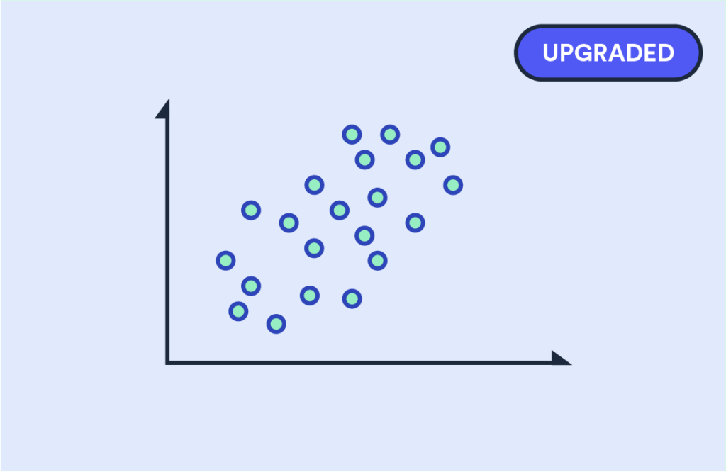
Scatterplots can help you visualize the data points and their assigned cluster labels by showing you the grouping patterns and the separation between clusters. Each data point is represented as a dot, and the different clusters are distinguished by different colors or symbols.

Use can also heatmaps to visualize the similarity or dissimilarity between data points and clusters. A heatmap displays a color-coded matrix, where each cell represents the distance or similarity measure between a data point and a cluster centroid. This visualization helps to identify which data points belong strongly to a particular cluster.

As mentioned earlier, dendrograms are common outputs from hierarchical cluster analyses. These show the merging or splitting of clusters at each step and can help you identify the hierarchical structure of the clusters and identify relationships between them.

Dimensionality reduction techniques

Applying dimensionality reduction techniques, such as principal component analysis (PCA) or t-SNE, can assist you to visualize the clusters in a lower-dimensional space. This can help reveal complex relationships and separations between clusters that are not easily visible in the original high-dimensional data.

Common Mistakes and Disadvantages with Cluster Analysis

Here are some common mistakes with cluster analysis to avoid.

Overfitting and underfitting

In cluster analysis, overfitting refers to the phenomenon where a clustering algorithm creates clusters that are overly complex or intricate, fitting the noise or idiosyncrasies of the data rather than capturing the underlying patterns or structure. Overfitting can occur when the algorithm has too much flexibility or when the number of clusters is too large compared to the intrinsic structure of the data.

Signs of overfitting in cluster analysis may include:

• Clusters that appear excessively fragmented or contain only a few data points.
• Clusters that exhibit irregular shapes or boundaries that do not align with the underlying structure of the data.
• Extremely fine-grained clusters that do not provide meaningful insights.

Underfitting in cluster analysis also means that the clustering algorithm has failed to capture patterns or the structure of the data adequately, but in this case it occurs when the chosen algorithm or settings are too rigid or simplistic to capture the complexity of the data.

Signs of underfitting in cluster analysis may include:

• Clusters that are overly generalized and fail to capture meaningful subgroups or distinctions.
• Inadequate separation between clusters, making it difficult to interpret or differentiate them. Clusters that do not align with known patterns or expectations in the data.

Underfitting can result in oversimplified or incomplete representations of the data.

Selection bias

One of the common mistakes or disadvantages to using cluster analysis is selection bias. When using hierarchical clustering, you need to make certain decisions when specifying both the distance metric and the linkage criteria. Unfortunately, there is rarely a strong theoretical basis for these decisions and such, can be described as arbitrary decisions. These decisions can lead to selection bias, which in turn leads to skewed or inaccurate clustering results.

Here are some scenarios where selection bias can occur in relation to cluster analysis:

• Non-random sampling: If the data used for clustering is collected through non-random sampling methods, such as convenience sampling or self-selection, it may introduce biases. For example, if participants self-select to be part of a study, their characteristics or behaviors may differ from those who did not volunteer, leading to biased clusters.
• Missing data bias: One disadvantage of cluster analysis is that most hierarchical clustering software will not work if you have missing data. However, if missing data is not handled appropriately, it can introduce selection bias. If certain individuals or variables have missing values that are not missing completely at random (MCAR), the clustering results may be distorted, as the missing data patterns could be related to the underlying cluster structure.
• Cluster selection bias: In hierarchical clustering, where clusters are formed through a stepwise merging process, the order in which the clusters are combined can impact the final results. If the order is biased or predetermined based on specific criteria, it can introduce selection bias and affect the resulting clusters.
• Exclusion of certain groups: If certain groups or subpopulations are excluded or underrepresented in the data used for clustering, the resulting clusters may not adequately capture the full diversity or patterns in the population. This can lead to incomplete or biased insights.

Best Practices for Cluster Analysis

Choosing appropriate distance metrics

Choosing an appropriate distance metric is a critical step in cluster analysis as it determines how similarity or dissimilarity is calculated between data points. The choice of distance metric should align with the characteristics of the data and the objectives of the clustering analysis. Here are some guidelines to consider when selecting distance metrics for cluster analysis:

• Understand the nature of the data: Consider the type of data you are working with. Is it numerical, categorical, binary, or a mix of different types? Different distance metrics are suitable for different types of data.
• Euclidean distance: Euclidean distance is commonly used for continuous or numerical data. It measures the straight-line distance between two points in Euclidean space. It assumes that all variables have equal importance and are on the same scale. Euclidean distance is widely used in algorithms like k-means and hierarchical clustering.
• Manhattan distance: Manhattan distance, also known as city block distance or L1 distance, calculates the sum of absolute differences between the coordinates of two points. It is appropriate for numerical data when the variables have different scales or represent different units. Manhattan distance is robust to outliers and is used in clustering algorithms like k-medians.
• Minkowski distance: Minkowski distance is a generalized distance metric that includes both Euclidean and Manhattan distances as special cases. It is defined as the nth root of the sum of the absolute values raised to the power of n. By varying the value of the parameter "n," different distance metrics can be obtained. When n=1, it is equivalent to Manhattan distance, and when n=2, it is equivalent to Euclidean distance.
• Hamming distance: Hamming distance is suitable for categorical or binary data. It measures the number of positions at which two strings of equal length differ. It is commonly used for clustering tasks involving text data, DNA sequences, or binary feature vectors.
• Jaccard distance: Jaccard distance is used to measure dissimilarity between sets. It is commonly used for binary or categorical data where presence or absence of items is of interest. Jaccard distance is defined as the ratio of the difference of the sizes of the intersection and union of two sets. It is often used in clustering tasks like text document clustering or item-based recommendation systems.

Selecting appropriate clustering algorithms

You also want to make sure that you select the appropriate clustering algorithms to align best with your data and objectives. Consider factors such as scalability, interpretability, and the ability to handle specific types of data (e.g., k-means for numerical data, DBSCAN for density-based clusters).

Evaluating cluster quality

Make sure you employ appropriate validation techniques to assess the quality of the clustering solution. Use both quantitative measures and visualizations to evaluate the cohesion, separation, and interpretability of the clusters. Some methods you can use include:

• Silhouette Coefficient: The silhouette coefficient measures how well each data point fits within its assigned cluster compared to other clusters. It ranges from -1 to +1, with higher values indicating better-defined and well-separated clusters.
• Davies-Bouldin Index: The Davies-Bouldin index evaluates the compactness and separation of clusters. It calculates the average dissimilarity between each cluster and its most similar cluster, with lower values indicating better clustering.
• Calinski-Harabasz Index: The Calinski-Harabasz index quantifies the ratio of between-cluster dispersion to within-cluster dispersion. Higher values suggest well-separated and compact clusters.

Future Directions in Cluster Analysis Research

Advancements in clustering algorithms

Researchers are continuously working on developing and improving clustering algorithms to address various challenges and data types. Some areas of advancement include:

• Robustness to high-dimensional data: As data dimensionality increases, clustering algorithms that can effectively handle high-dimensional data while preserving meaningful structures are being explored. Techniques such as subspace clustering, ensemble clustering, or sparse clustering are being developed to address this challenge.
• Scalability and efficiency: With the increasing size of datasets, scalable clustering algorithms are being developed to handle big data efficiently. Methods such as distributed clustering, online clustering, or parallel clustering algorithms are gaining attention to address scalability concerns.

Integration with other machine learning techniques

Cluster analysis is often combined with other machine learning techniques to improve the overall analysis and obtain more actionable insights. One integration direction includes integrating clustering with deep learning techniques. Approaches like deep clustering and autoencoders are being explored to combine deep learning and clustering.

Emerging applications and areas of research

Cluster analysis is finding applications in various domains, and researchers are exploring new areas of application and conducting domain-specific studies. Some emerging areas of research include:

• Healthcare and precision medicine: Clustering techniques are being used to identify patient subgroups, disease patterns, or personalized treatment approaches. Clustering is aiding in precision medicine initiatives by enabling better patient stratification and disease subtype discovery.
• Social network analysis: Clustering algorithms are employed in social network analysis to identify communities or detect influential nodes. Research focuses on developing algorithms that capture the dynamic nature of social networks and consider multiple network attributes.
• Anomaly detection and cybersecurity: Clustering techniques are used for anomaly detection, identifying outliers, or detecting network intrusions. Researchers are working on developing clustering algorithms that can handle complex and evolving threats in cybersecurity.
• Image and video analysis: Clustering methods are applied to image and video data for tasks such as image segmentation, object recognition, or video summarization. Research focuses on developing algorithms that can handle large-scale image and video datasets efficiently and capture complex visual patterns.

These are just a few examples of the future directions in cluster analysis research. As data and technology continue to evolve, cluster analysis will play a vital role in extracting meaningful information and insights from complex datasets across various domains.

Resources and Tools for Cluster Analysis

Software and programming languages for cluster analysis

Displayr
Displayr is an all-in-one analysis and reporting software purpose-built for researchers. It makes it easy to perform hierarchical clustering, k-means clustering, latent class analysis, and all the associated techniques for predicting class membership in new data sets (e.g., regression, machine learning). Displayr also automatically deals with missing data problems using the best-practice MAR assumption.

R
R is a popular open-source programming language and environment for statistical computing and data analysis. It provides a wide range of packages and libraries designed for cluster analysis, such as "stats," "cluster," "fpc," and "dbscan." R offers a comprehensive set of functions for performing various clustering algorithms, evaluating cluster validity, and visualizing clustering results.

Python
Python is a versatile programming language with a rich ecosystem of libraries and tools for data analysis and machine learning. The "scikit-learn" library in Python provides numerous clustering algorithms, including k-means, hierarchical clustering, DBSCAN, and more. Python also offers libraries like "scipy" and "numpy" that provide additional functions and tools for cluster analysis.

MATLAB
MATLAB is a proprietary programming language and development environment commonly used in scientific and engineering applications. It offers a wide range of functions and toolboxes for cluster analysis, including clustering algorithms, cluster validation metrics, and visualization capabilities. The Statistics and Machine Learning Toolbox in MATLAB provides several clustering algorithms and tools.

SPSS
SPSS (Statistical Package for the Social Sciences) is a software package for statistical analysis. It offers several clustering algorithms, including k-means, hierarchical clustering, and two-step clustering.

Data sources and datasets for practice

If you’d like to explore more about cluster analysis, you can try it yourself for free using Displayr or explore these examples of hierarchical cluster analysis on different datasets using R.

Learning resources

Looking to learn from more real world applications of cluster analysis? You can explore how to use cluster analysis for market segmentation with this eBook on How to do Market Segmentation or webinar on DIY Market Segmentation.